
// Modify here, bug causes nav to spill behind body on ultra large resolutions
In this guide you will be able to visualize college enrollment rates by high school, college type, student achievement level before high school, student race/ethnicity, and combinations of these factors. You will also be able to visualize the share of highly qualified students who enroll in selective colleges.
The College-Going Pathways series is a set of guides, code, and sample data about policy-relevant college-going topics. Browse this and other guides in the series for ideas about ways to investigate student pathways through high school and college. Each guide includes several analyses in the form of charts together with Stata analysis and graphing code to generate each chart.
Once you’ve identified analyses that you want to try to replicate or modify, click the “Download” buttons to download Stata code and sample data. You can make changes to the charts using the code and sample data, or modify the code to work with your own data. If you’re familiar with Github, you can click “Go to Repository” and clone the entire College-Going Pathways repository to your own computer.
The data visualizations in the College-Going Pathways series use a synthetically generated college-going analysis sample data file which has one record per student. Each high school student is assigned to a ninth-grade cohort, and each student record includes demographic and program participation information, annual GPA and on-track status, high school graduation outcomes, and college enrollment information. The Connect guide (coming soon) will provide guidance and example code which will help you build a college-going analysis file using data from your own school system.
Given the substantial economic and social benefits of a college degree, understanding a high schools’ role in preparing students to persist through college is essential. This section provides a series of analyses that highlight college-going rates across high schools in your agency. You will consider whether high school graduates enroll in colleges and universities well-aligned to their incoming academic qualifications. This is one factor that may increase a students’ likelihood of college persistence and degree attainment.
One of the most important decisions in running each analysis is defining the sample. Each analysis corresponds to a different part of the education pipeline and as a result requires different cohorts of students.
If you are using the synthetic data we have provided, the sample restrictions have been predefined and are included below. If you run this code using your own agency data, change the sample restrictions based on your data. Note that you will have to run these sample restrictions at the beginning of your do file so they will feed into the rest of your code.
// Sample Restrictions

// Agency name
global agency_name "Agency"

// Ninth grade cohorts you can observe persisting to the second year of college
global chrt_ninth_begin_persist_yr2 = 2004
global chrt_ninth_end_persist_yr2 = 2006

// Ninth grade cohorts you can observe graduating high school on time
global chrt_ninth_begin_grad = 2004
global chrt_ninth_end_grad = 2006

// Ninth grade cohorts you can observe graduating high school one year late
global chrt_ninth_begin_grad_late = 2004
global chrt_ninth_end_grad_late = 2006

// High school graduation cohorts you can observe enrolling in college the fall after graduation
global chrt_grad_begin = 2007
global chrt_grad_end = 2009

// High school graduation cohorts you can observe enrolling in college two years after hs graduation
global chrt_grad_begin_delayed = 2007
global chrt_grad_end_delayed = 2009
Based on the sample data, you will have three cohorts (sometimes only two) for analysis. If you are using your own agency data, you may decide to aggregate results for more or fewer cohorts to report your results. This decision depends on 1) how much historical data you have available and 2) what balance to strike between reliability and averaging away information on recent trends. We suggest you average results for the last three cohorts to take advantage of larger sample sizes and improve reliability. However, if you have data for more than three cohorts, you may decide to not average data out for fear of losing information about trends and recent changes in your agency.
This guide is an open-source document hosted on Github and generated using the Stata Webdoc package. We welcome feedback, corrections, additions, and updates. Please visit the OpenSDP college-going pathways repository to read our contributor guidelines.
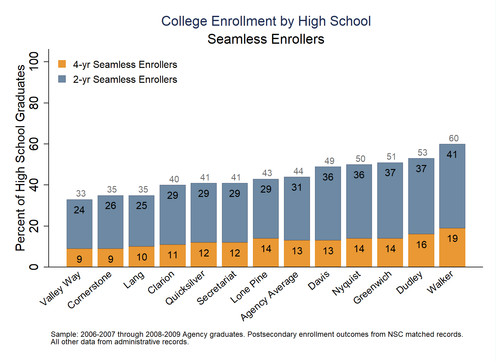
Purpose: This analysis provides an agency snapshot of college enrollment to understand how patterns of college going for high school graduates vary across high schools. By illuminating the extent to which enrollment varies by entry time for seamless enrollers and college level (2- vs. 4-year), the analysis helps diagnose compositional differences for the college-bound population by high school attended.
Required Analysis File Variables:
sidchrt_gradenrl_1oct_grad_yr1_anyenrl_1oct_grad_yr1_2yrenrl_1oct_grad_yr1_4yrenrl_ever_w2_grad_2yrenrl_ever_w2_grad_4yrhs_diplomalast_hs_codelast_hs_nameAnalysis-Specific Sample Restrictions:
Ask Yourself - How do college enrollment rates differ by high schools? Why might certain schools have a greater percentage of high school graduates enrolling in college? Do certain schools have higher percentages of 2-year or delayed college enrollers?
Possible Next Steps or Action Plans: Replicate this analysis to include all first-time ninth graders (i.e. ninth grade cohorts) in place of graduates. Additionally, create individual high school reports that provide more details for school administrators (top enrolling institutions of the school’s graduates).
Analytic Technique: Calculate the proportion of students who enroll in college by high school.
// College Enrollment Rates by High School

// Step 1:  Load the college-going analysis file into Stata
use "$data/college_going_analysis", clear

// Step 2: Keep students in high school graduation cohorts you can observe enrolling in college the fall after graduation
local chrt_grad_begin = ${chrt_grad_begin}
local chrt_grad_end = ${chrt_grad_end}
keep if (chrt_grad >= `chrt_grad_begin' & chrt_grad <= `chrt_grad_end')

// Step 3: Obtain the agency-level average for seamless enrollment
preserve
    collapse (sum) enrl_1oct_grad_yr1_2yr enrl_1oct_grad_yr1_4yr hs_diploma
    tempfile agency_level
    save `agency_level'
restore

// Step 4: Obtain the school-level averages for seamless enrollment and append on the agency average.
collapse (sum) enrl_1oct_grad_yr1_2yr enrl_1oct_grad_yr1_4yr hs_diploma, by(last_hs_name last_hs_code)
append using `agency_level'

// Step 5: Provide a hs name label for the appended agency average and shorten hs name
replace last_hs_name = "${agency_name} Average" if mi(last_hs_name)
replace last_hs_code = 0 if mi(last_hs_code)
replace last_hs_name = subinstr(last_hs_name, " High School", "", .)

// Step 6: Generate percentages of high school grads attending college. Multiply outcomes of interest by 100 for graphical representations of the rates
foreach var of varlist enrl_1oct_grad_yr1_* {
    gen pct_`var' = `var' / hs_diploma
    replace pct_`var' = round((pct_`var' * 100))
}

// Step 7: Create a total seamless college enrollment rates by summing up the other variables
gen total_seamless = pct_enrl_1oct_grad_yr1_2yr + pct_enrl_1oct_grad_yr1_4yr

// Step 8: Prepare to graph the results
// 1. Generate a cohort label to be used in the footnote for the graph
local temp_begin = `chrt_grad_begin'-1
local temp_end = `chrt_grad_end'-1
if `chrt_grad_begin'==`chrt_grad_end' {
    local chrt_label "`temp_begin'-`chrt_grad_begin'"
}
else {
    local chrt_label "`temp_begin'-`chrt_grad_begin' through `temp_end'-`chrt_grad_end'"
}

// 2. Generate graphing code to place value labels for the total enrollment rates; change xpos (the position of the first leftmost label) and xposwidth (the horizontal width of the labels) to finetune.
sort total_seamless
local total_seamless ""
local num_obs = _N
foreach n of numlist 1/`num_obs' {
    local temp_total_seamless = total_seamless in `n'
    local total_seamless "`total_seamless' `temp_total_seamless'"
}
local total_seamless_label ""
local xpos = 4.8
local xposwidth = 98.7
foreach val of local total_seamless {
    local val_pos = `val' + 3
    local total_seamless_label `"`total_seamless_label' text(`val_pos' `xpos' "`val'", size(2.5) color(gs7))"'
    local xpos = `xpos' + `xposwidth'/_N
}
disp `"`total_seamless_label'"'

// Step 9: Graph the results
#delimit ;
graph bar pct_enrl_1oct_grad_yr1_4yr  pct_enrl_1oct_grad_yr1_2yr
    if hs_diploma >= 20, stack over(last_hs_name, label(angle(40) labsize(small)) gap(20) sort(total_seamless))
    bar(1, fcolor(dkorange) fi(inten80) lcolor(dkorange) lwidth(vvvthin))
    bar(2, fcolor(navy*.8) fi(inten80) lcolor(dknavy*.8) lwidth(vvvthin))
    blabel(bar, position(inside) color(black) size(small))
legend(label(1 "4-yr Seamless Enrollers")
    label(2 "2-yr Seamless Enrollers")
    position(11) ring(0) symxsize(2) symysize(2) rows(2) size(small) region(lstyle(none) lcolor(none) color(none)))
title("College Enrollment by High School", size(medium))
    ytitle("Percent of High School Graduates")
    subtitle("Seamless Enrollers")
    `total_seamless_label'
    yscale(range(0(20)100))
    ylabel(0(20)100, nogrid)
graphregion(color(white) fcolor(white) lcolor(white))
plotregion(color(white) fcolor(white) lcolor(white))
note("Sample: `chrt_label' ${agency_name} graduates. Postsecondary enrollment outcomes from NSC matched records." "All other data from administrative records.", size(vsmall));
#delimit cr

graph export "figures/D1_Col_Enrl_Seamless_by_HS.png", replace width(1600) height(1200)
Purpose: This analysis provides an agency snapshot of college enrollment to understand how patterns of college going for high school graduates vary across high schools. By illuminating the extent to which enrollment varies by entry time (seamless vs. delayed) and college level (2- vs. 4-year), the analysis helps diagnose compositional differences for the college-bound population by high school attended.
Required Analysis File Variables:
sidchrt_gradenrl_1oct_grad_yr1_anyenrl_1oct_grad_yr1_2yrenrl_1oct_grad_yr1_4yrenrl_ever_w2_grad_2yrenrl_ever_w2_grad_4yrhs_diplomalast_hs_codelast_hs_nameAnalysis-Specific Sample Restrictions:
Ask Yourself
Possible Next Steps or Action Plans: Replicate this analysis to include all first-time ninth graders (i.e. ninth grade cohorts) in place of graduates. Additionally, create individual high school reports that provide more details for school administrators (top enrolling institutions of the school’s graduates).
Analytic Technique: Calculate the proportion of graduates who enroll in four-year institutions across high schools according to the selectivity ranking of the postsecondary institutions attended.
// Seamless and Delayed College Enrollment Rates by High School

if 0 {
// Step 1: Load the college-going analysis file into Stata
use "$data/college_going_analysis", clear

// Step 2: Keep students in high school graduation cohorts you can observe enrolling in college the fall after graduation
local chrt_grad_begin = ${chrt_grad_begin}
local chrt_grad_end = ${chrt_grad_end}
keep if (chrt_grad >= `chrt_grad_begin' & chrt_grad <= `chrt_grad_end')

// Step 3: Create binary outcomes for late enrollers
gen late_any = enrl_1oct_grad_yr1_any==0 & enrl_ever_w2_grad_any==1
gen late_4yr = enrl_1oct_grad_yr1_any==0 & enrl_ever_w2_grad_4yr==1
gen late_2yr = enrl_1oct_grad_yr1_any==0 & enrl_ever_w2_grad_2yr==1
assert late_4yr + late_2yr == late_any

// Step 4: Obtain the agency average for seamless and delayed enrollment
preserve
    collapse (sum) enrl_1oct_grad_yr1_2yr enrl_1oct_grad_yr1_4yr late_4yr late_2yr hs_diploma
    tempfile agency_level
    save `agency_level'
restore

// Step 4: Obtain the school-level averages for seamless and delayed enrollment and append on the agency average
collapse (sum) enrl_1oct_grad_yr1_2yr enrl_1oct_grad_yr1_4yr late_4yr late_2yr hs_diploma, by(last_hs_name last_hs_code)
append using `agency_level'

// Step 5: Provide a hs name label for the appended agency average and shorten hs name
replace last_hs_name = "${agency_name} Average" if mi(last_hs_name)
replace last_hs_code = 0 if mi(last_hs_code)
replace last_hs_name = subinstr(last_hs_name, " High School", "", .)

// Step 6: Generate percentages of high school grads attending college. Multiply outcomes of interest by 100 for graphical representations of the rates
foreach var of varlist enrl_1oct_grad_yr1_* late_* {
    gen pct_`var' = `var' / hs_diploma
    replace pct_`var' = round((pct_`var' * 100))
}

// Step 7: Create total college enrollment rates by summing up the other variables; you can add additional labels as you see fit
gen total = pct_enrl_1oct_grad_yr1_2yr + pct_enrl_1oct_grad_yr1_4yr + pct_late_4yr + pct_late_2yr
gen total_seamless = pct_enrl_1oct_grad_yr1_2yr + pct_enrl_1oct_grad_yr1_4yr

// Step 8: Prepare to graph the results
// Generate a cohort label to be used in the footnote for the graph
local temp_begin = `chrt_grad_begin'-1
local temp_end = `chrt_grad_end'-1
if `chrt_grad_begin'==`chrt_grad_end' {
    local chrt_label "`temp_begin'-`chrt_grad_begin'"
}
else {
    local chrt_label "`temp_begin'-`chrt_grad_begin' through `temp_end'-`chrt_grad_end'"
}

// Step 9: Graph the results
#delimit ;
graph bar pct_enrl_1oct_grad_yr1_4yr pct_late_4yr pct_enrl_1oct_grad_yr1_2yr pct_late_2yr
    if hs_diploma >= 20, over(last_hs_name, label(angle(40)labsize(small)) gap(20) sort(total))
    bar(1, fcolor(dkorange) fi(inten80) lcolor(dkorange) lwidth(vvvthin))
    bar(2, fcolor(dkorange*.4) fi(inten80) lcolor(dkorange*.4) lwidth(vvvthin))
    bar(3, fcolor(navy*.8) fi(inten80) lcolor(navy*.8) lwidth(vvvthin))
    bar(4, fcolor(navy*.4) fi(inten30) lcolor(navy*.4) lwidth(vvvthin)) stack
    blabel(bar, position(inside) color(black) size(small))
legend(label(1 "4-yr Seamless")
    label(2 "4-yr Delayed")
    label(3 "2-yr Seamless")
    label(4 "2-yr Delayed")
    position(11) order(4 3 2 1) ring(0) symxsize(2) symysize(2) rows(4) size(small) region(lstyle(none) lcolor(none) color(none)))
title("College Enrollment by High School", size(medium))
    ytitle("Percent of High School Graduates")
    subtitle("Seamless and Delayed Enrollers")
    yscale(range(0(20)100))
    ylabel(0(20)100, nogrid)
graphregion(color(white) fcolor(white) lcolor(white))
plotregion(color(white) fcolor(white) lcolor(white))
note("Sample: `chrt_label' ${agency_name} graduates."
"Postsecondary enrollment outcomes from NSC matched records. All other data from administrative records.", size(vsmall));
#delimit cr

graph export "figures/D2_Col_Enrl_Seamless_Delayed_by_HS.png", replace width(1600) height(1200)
}
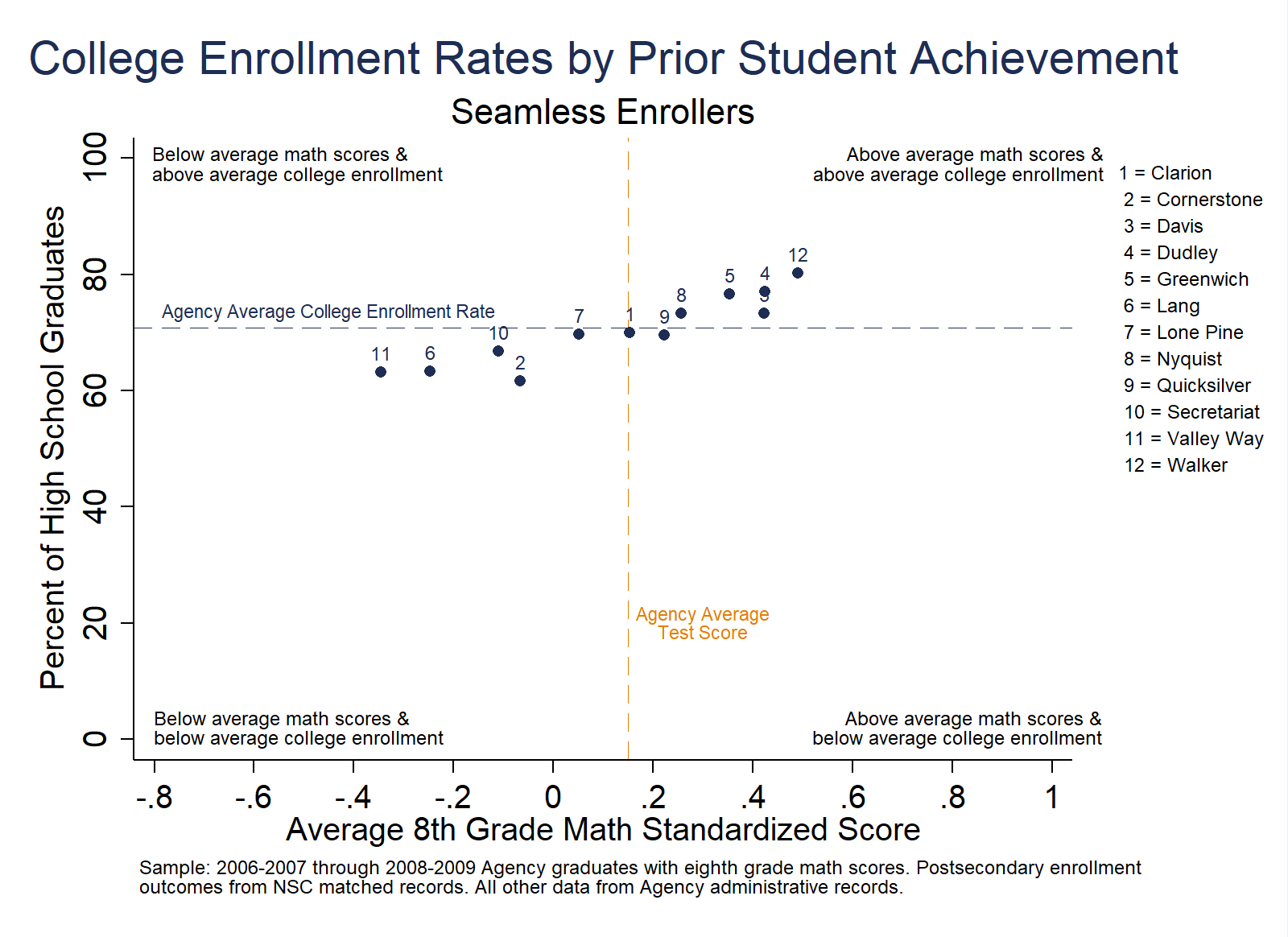
Purpose: This analysis displays variations in college enrollment rates across high schools by examining the extent to which academic achievement at high school entry explains variation in college going across high schools. This analysis is useful to identify high schools with similar incoming student achievement profiles but divergent college enrollment rates; or on the other hand, high schools with similar college-going rates but different academic performance at high school entry.
Required Analysis File Variables:
sidchrt_gradenrl_1oct_grad_yr1_anytest_math_8_stdlast_hs_codelast_hs_nameAnalysis-Specific Sample Restrictions:
Ask Yourself - What might explain variation in college enrollment rates for high schools with similar incoming achievement? What might explain variation in incoming achievement for high schools with similar college enrollment rates?
Possible Next Steps or Action Plans: Repeat this analysis to include all first-time ninth graders (i.e. ninth grade cohorts) in place of graduates, and explore college enrollment within two years of high school completion. Additionally, replicate this analysis to explore the relationship between college enrollment and students’ ELA achievement at high school entry. Consider why schools with similar incoming student profiles may report dramatically different college-going rates. Conversely, consider why schools with dissimilar student bodies report similar matriculation rates to college.
Analytic Technique: Bivariate scatterplot of school-level average student test scores and college enrollment rates.
// College Enrollment Rates by Average 8th Grade Achievement

// Step 1: Load the college-going analysis file into Stata
use "$data/college_going_analysis", clear

// Step 2: Keep students in high school graduation cohorts you can observe enrolling in college the fall after graduation AND have non-missing eighth grade math scores
local chrt_grad_begin = ${chrt_grad_begin}
local chrt_grad_end = ${chrt_grad_end}
keep if (chrt_grad >= `chrt_grad_begin' & chrt_grad <= `chrt_grad_end') & !mi(test_math_8_std)

// Step 3: Obtain agency-level college enrollment rate and prior achievement score along with the position of their labels.
summ enrl_1oct_grad_yr1_any
local agency_mean_enroll = `r(mean)'*100
local agency_mean_enroll_label = `agency_mean_enroll' + 3
summ test_math_8_std
local agency_mean_test = `r(mean)'
local agency_mean_test_label = `agency_mean_test' + 0.15

// Step 4: Obtain school-level college enrollment rates and prior achievement scores
collapse (mean) test_math_8_std enrl_1oct_grad_yr1_any (count) N = sid, by(last_hs_code last_hs_name)

// Step 5: Multiply the college enrollment rate by 100 for graphical representation of the rates
replace enrl_1oct_grad_yr1_any = round((enrl_1oct_grad_yr1_any * 100), .1)

// Step 6: Shorten high school names and create a legend label for the graph
sort last_hs_name
replace last_hs_name = subinstr(last_hs_name, " High School", "", .)
gen hs_code_label = _n
levelsof last_hs_name, local(hs_names)
local count = 1
local legend_labels ""
foreach hs of local hs_names {
    local legend_labels `"`legend_labels' `count' = `hs'"' `" "'
    local ++count
}

// Step 7: Prepare to graph the results
// Generate a cohort label to be used in the footnote for the graph
local temp_begin = `chrt_grad_begin'-1
local temp_end = `chrt_grad_end'-1
if `chrt_grad_begin'==`chrt_grad_end' {
    local chrt_label "`temp_begin'-`chrt_grad_begin'"
}
else {
    local chrt_label "`temp_begin'-`chrt_grad_begin' through `temp_end'-`chrt_grad_end'"
}

// Step 8: Graph the results
#delimit ;
twoway (scatter enrl_1oct_grad_yr1_any test_math_8_std, mlabel(hs_code_label) mlabsize(vsmall)
    mlabposition(12) mlabcolor(dknavy) mstyle(x) msize(small) mcolor(dknavy)),
title("College Enrollment Rates by Prior Student Achievement")
    subtitle("Seamless Enrollers")
    xtitle("Average 8th Grade Math Standardized Score", linegap(0.3))
    ytitle("Percent of High School Graduates" " ")
xscale(range(-0.8(0.2)1)) xlabel(-0.8(0.2)1)
yscale(range(0(20)100)) ylabel(0(20)100, nogrid)
legend(on order(3) col(1) label(3 `"`legend_labels'"')
    region(color(none)) size(vsmall) position(2) ring(1) linegap(.75))
    yline(`agency_mean_enroll', lpattern(dash) lcolor(dknavy) lwidth(vvthin))
    xline(`agency_mean_test', lpattern(dash) lcolor(dkorange) lwidth(vvthin))
text(`agency_mean_enroll_label' -0.45 "${agency_name} Average College Enrollment Rate", size(2.0) color(dknavy))
text(20 `agency_mean_test_label' "${agency_name} Average" "Test Score", size(2.0) color(dkorange))
text(99 -0.5 "Below average math scores &" "above average college enrollment",
    size(vsmall) justification(left))
text(99 0.8 "Above average math scores &" "above average college enrollment",
    size(vsmall) justification(right))
text(2 -0.5 "Below average math scores &" "below average college enrollment",
    size(vsmall) justification(left))
text(2 0.8 "Above average math scores &" "below average college enrollment",
    size(vsmall) justification(right))
graphregion(color(white) fcolor(white) lcolor(white))
plotregion(color(white) fcolor(white) lcolor(white))
note("Sample: `chrt_label' ${agency_name} graduates with eighth grade math scores. Postsecondary enrollment"
"outcomes from NSC matched records. All other data from ${agency_name} administrative records.", size(vsmall));
#delimit cr

graph export "figures/D3_Col_Enrl_by_Avg_Eighth.png", replace width(1600) height(1200)
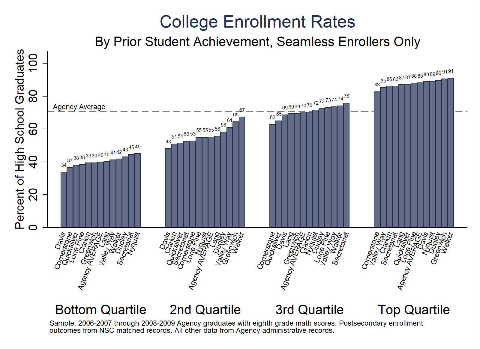
Purpose: This analysis explores whether variation in college enrollment across high schools is similar among low-, middle, and top-achieving students. It also considers whether overall variation across schools derives from concentrated divergence among students scoring in a particular achievement range. Additionally, the analysis facilitates granular school-to-school comparisons to identify those especially under-, or over-performing within each achievement quartile. Finally, the analysis also helps identify which student subgroups require additional resources and support within each school.
Required Analysis File Variables:
sidchrt_gradenrl_1oct_grad_yr1_anyqrt_8_math_stdlast_hs_codelast_hs_nameAnalysis-Specific Sample Restrictions:
Ask Yourself
Possible Next Steps or Action Plans: Repeat this analysis to include all first-time ninth graders (i.e. ninth grade cohorts) in place of graduates, and explore college enrollment within two years of high school completion. Additionally, replicate this analysis to explore the relationship between college enrollment and students’ ELA achievement at high school entry. Consider why schools with similar incoming student profiles may report dramatically different college-going rates. Conversely, consider why schools with distinct student bodies may report similar matriculation rates to college.
Analytic Technique: Calculate the proportion of graduates who enrolled in college by October 1st following their high school graduation year by high school and 8th grade test score quartile.
// College Enrollment Rates by 8th Grade Achievement Quartiles

// Step 1: Load the college-going analysis file into Stata
use "$data/college_going_analysis", clear

// Step 2: Keep students in high school graduation cohorts you can observe enrolling in college the fall after graduation AND have non-missing eighth grade math scores
local chrt_grad_begin = ${chrt_grad_begin}
local chrt_grad_end = ${chrt_grad_end}
keep if (chrt_grad >= `chrt_grad_begin' & chrt_grad <= `chrt_grad_end') & !mi(qrt_8_math)

// Step 3: Obtain the overall agency-level high school graduation rate along with the position of its label.
summ enrl_1oct_grad_yr1_any
local agency_mean = `r(mean)'*100
local agency_mean_label = `agency_mean'+3

// Step 4: Obtain the agency-level college enrollment rate by test score quartile
preserve
    collapse (mean) enrl_1oct_grad_yr1_any (count) N = sid, by(qrt_8_math)
    tempfile agency_level
    save `agency_level'
restore

// Step 5: Obtain school-level college enrollment rates by test score quartile and append the agency-level enrollment rates by quartile
collapse (mean) enrl_1oct_grad_yr1_any (count) N = sid, by(last_hs_code last_hs_name qrt_8_math)
append using `agency_level'

// Step 6: Shorten high school names and drop any high schools with fewer than 20 students
replace last_hs_code = 0 if last_hs_code == .
replace last_hs_name = "${agency_name} AVERAGE" if mi(last_hs_name)
replace last_hs_name = subinstr(last_hs_name, " High School", "", .)
drop if N < 20

// Step 7: Multiply the college enrollment rate by 100 for graphical representation of the rates
replace enrl_1oct_grad_yr1_any = round((enrl_1oct_grad_yr1_any * 100), .1)

// Step 8: Create a variable to sort schools within each test score quartile in ascending order
sort qrt_8_math enrl_1oct_grad_yr1_any
gen rank = _n

// Step 9: Prepare to graph the results
// Generate a cohort label to be used in the footnote for the graph
local temp_begin = `chrt_grad_begin'-1
local temp_end = `chrt_grad_end'-1
if `chrt_grad_begin'==`chrt_grad_end' {
    local chrt_label "`temp_begin'-`chrt_grad_begin'"
}
else {
    local chrt_label "`temp_begin'-`chrt_grad_begin' through `temp_end'-`chrt_grad_end'"
}

// Step 10: Graph the results
#delimit ;
graph bar enrl_1oct_grad_yr1_any, over(last_hs_name, sort(rank) gap(0) label(angle(70) labsize(vsmall)))
    over(qrt_8_math, relabel(1 "Bottom Quartile" 2 "2nd Quartile" 3 "3rd Quartile" 4 "Top Quartile") gap(400))
    bar(1, fcolor(dknavy) finten(70) lcolor(dknavy) lwidth(thin))
    blabel(bar, position(outside) format(%8.0f) size(tiny))
    yscale(range(0(20)100))
    ylabel(0(20)100, nogrid)
legend(off)
title("College Enrollment Rates")
    subtitle("By Prior Student Achievement, Seamless Enrollers Only", size(msmall))
    ytitle("Percent of High School Graduates")
    yline(`agency_mean', lpattern(dash) lwidth(vvthin) lcolor(dknavy))
text(`agency_mean_label' 5 "${agency_name} Average", size(vsmall))
graphregion(color(white) fcolor(white) lcolor(white))
plotregion(color(white) fcolor(white) lcolor(white))
note("Sample: `chrt_label' ${agency_name} graduates with eighth grade math scores. Postsecondary enrollment" "outcomes from NSC matched records. All other data from ${agency_name} administrative records.", size(vsmall));
#delimit cr

graph export "figures/D4_Col_Enrl_by_Eighth_Qrt.png", replace width(1600) height(1200)
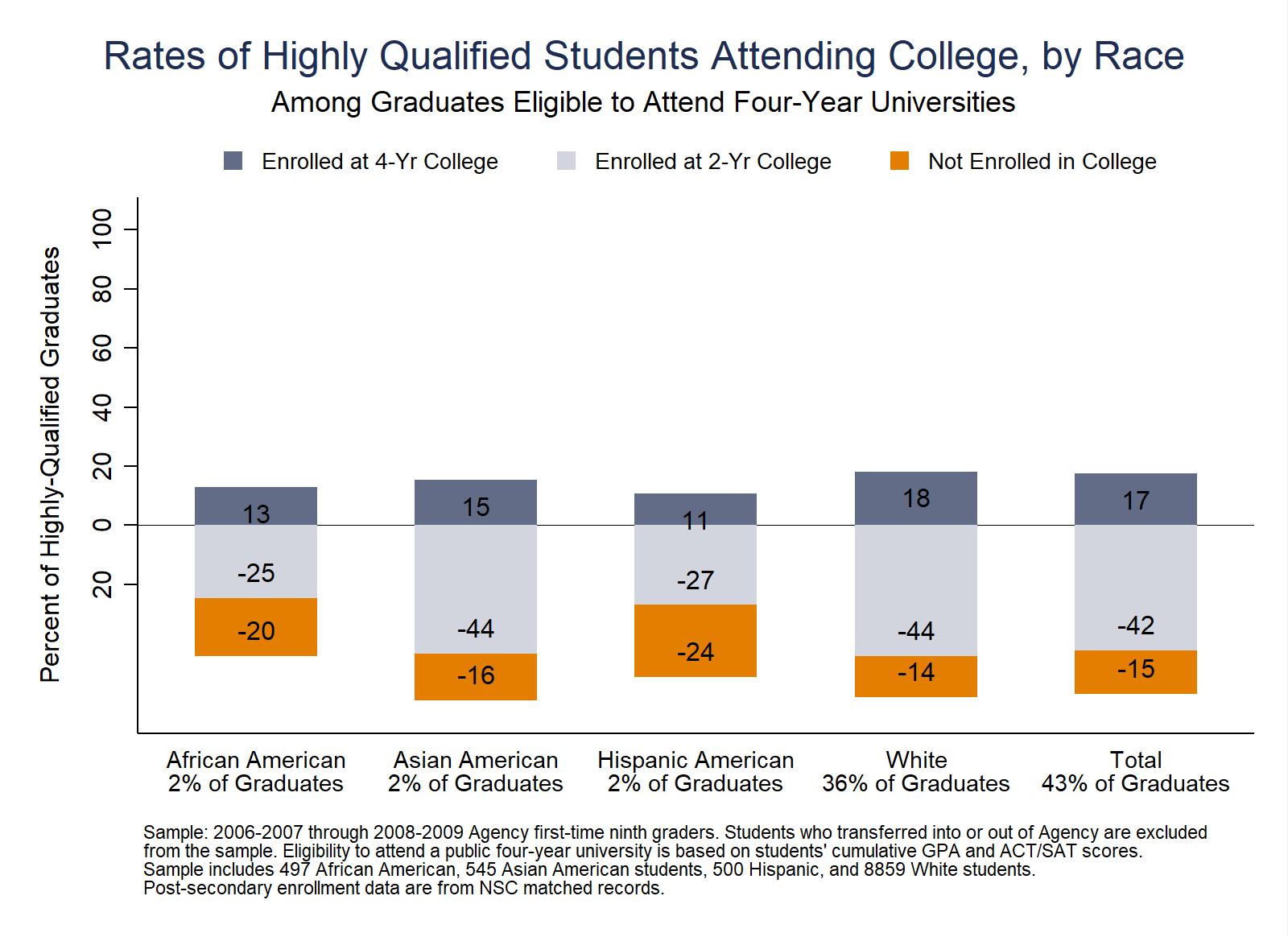
Purpose: Research consistently finds wide variation in rates of persistence and completion across postsecondary institutions. This analysis examines whether high school graduates enroll in colleges and universities that provide the right academic fit to maximize their chances of completion. “Match”describes the extent high school graduates with strong academic records attend colleges and universities that allow them to take advantage of their ambition and abilities. While “matching” to an appropriately selective college is only one factor to consider when choosing a postsecondary institution, the implications of under-matching (i.e. lower rates of persistence and degree completion) suggest students should be encouraged to attend realistic, yet challenging postsecondary institutions.
Required Analysis File Variables:
sidrace_ethnicitychrt_gradhighly_qualifiedenrl_1oct_grad_yr1_anyenrl_1oct_grad_yr1_4yrenrl_1oct_grad_yr1_2yrAnalysis-Specific Sample Restrictions:
Ask Yourself
Possible Next Steps or Action Plans: This analysis leads to important questions that warrant further exploration. What factors drive undermatch differences across student subgroups and high schools? To what extent is undermatching concentrated among first-time college-goers? To what extent is undermatching driven by students’ proximity to 2-year versus 4-year institutions? What college aspirations do incoming ninth graders hold, and do these aspirations change by the time they enter or complete 12th grade? To what extent are teachers, counselors, and administrators supported to work with students to cultivate postsecondary aspirations and weigh factors in the college selection process?
Analytic Technique: Calculate the proportion of highly qualified graduates who do not enroll in college, enroll in 2-year college, and enroll in least competitive and unranked 4-year colleges the fall following high school graduation.
// Rates of College Enrollment by College Type Among Highly Qualified Graduates

// Step 1: Load the college-going analysis file into Stata
use "$data/college_going_analysis", clear

// Step 2: Keep students in high school graduation cohorts you can observe enrolling in college the fall after graduation
local chrt_grad_begin = ${chrt_grad_begin}
local chrt_grad_end = ${chrt_grad_end}
keep if (chrt_grad >= `chrt_grad_begin' & chrt_grad <= `chrt_grad_end')

// Step 3: Get total number of students in sample
gen total_count = _N

// Step 4: Further restrict sample to include only highly qualified students
keep if highly_qualified == 1

// Step 5: Create "undermatch" outcomes
gen no_college = (enrl_1oct_grad_yr1_any == 0)
gen enrl_2yr = (enrl_1oct_grad_yr1_2yr == 1)
gen enrl_4yr = (enrl_1oct_grad_yr1_4yr == 1)

// Step 6: Create agency-level outcomes for total undermatching rates
preserve
    collapse (mean) no_college enrl_2yr enrl_4yr total_count (count) N = sid
    gen group = 5
    tempfile total
    save `total'
restore

// Step 7: Create race/ethnicity-level outcomes for undermatching rates by race/ethnicity
collapse (mean) no_college enrl_2yr enrl_4yr total_count (count) N = sid , by(race_ethnicity)
append using `total'
replace group = 1 if race_ethnicity==1
replace group = 2 if race_ethnicity==2
replace group = 3 if race_ethnicity==3
replace group = 4 if race_ethnicity==5
drop if mi(group)

// Step 8: Multiply the college enrollment rate by 100 for graphical representation of the rates
foreach v of varlist no_college enrl_2yr enrl_4yr {
    replace `v' = round(`v'*100, .1)
}

// Step 9: Multiply the outcome variables corresponding to undermatching by "-1" to visually display these rates as negative values
foreach var of varlist no_college enrl_2yr {
    replace `var' = `var'*-1
}

// Step 10: Prepare to graph the results
// 1. Create labels for numbers in graph
gen pct_total = N/total_count
sort group
local numobs = _N
foreach v of numlist 1/`numobs' {
    local pct_`v' = round(pct_total*100) in `v'
    local count_`v' = N in `v'
}
// 2. Generate a cohort label to be used in the footnote for the graph
local temp_begin = `chrt_grad_begin'-1
local temp_end = `chrt_grad_end'-1
if `chrt_grad_begin'==`chrt_grad_end' {
    local chrt_label "`temp_begin'-`chrt_grad_begin'"
}
else {
    local chrt_label "`temp_begin'-`chrt_grad_begin' through `temp_end'-`chrt_grad_end'"
}

// Step 11: Graph the results
#delimit ;
graph bar enrl_4yr enrl_2yr no_college, stack over(group,
    relabel(1 `""African American" "`pct_1'% of Graduates""' 2 `""Asian American" "`pct_2'% of Graduates""' 3 `""Hispanic American" "`pct_3'% of Graduates""' 4 `""White" "`pct_4'% of Graduates""' 5 `""Total" "`pct_5'% of Graduates""')
    label(labsize(2.5)) gap(80)) blabel(bar, format(%9.0f) size(small) position(inside) color(black))
    bar(1, fcolor(dknavy*.7) lcolor(dknavy*.7) lwidth(vvthin))
    bar(2, fcolor(dknavy*.2) lcolor(dknavy*.2) lwidth(vvthin))
    bar(3, fcolor(dkorange) lcolor(dkorange) lwidth(vvthin))
    yscale(range(-20(20)100))
    ylabel(-20(20)100, nogrid labsize(small))
    ylabel(-20 "20" 0 "0" 20 "20" 40 "40" 60 "60" 80 "80" 100 "100")
    yline(0, lcolor(black) lwidth(vvthin))
title("Rates of Highly Qualified Students Attending College, by Race", size(medlarge) span)
    subtitle("Among Graduates Eligible to Attend Four-Year Universities", size(*.8) span)
    ytitle("Percent of Highly-Qualified Graduates" " ", size(small))
legend(region(lcolor(white)) position(12) row(1) label(1 "Enrolled at 4-Yr College")
    label(2 "Enrolled at 2-Yr College") label(3 "Not Enrolled in College") symxsize(2) symysize(2) size(*.7))
    graphregion(color(white) fcolor(white) lcolor(white))
    plotregion(color(white) fcolor(white) lcolor(white))
note(" " "Sample: `chrt_label' ${agency_name} first-time ninth graders. Students who transferred into or out of ${agency_name} are excluded"
"from the sample. Eligibility to attend a public four-year university is based on students' cumulative GPA and ACT/SAT scores."
"Sample includes `count_1' African American, `count_2' Asian American students, `count_3' Hispanic, and `count_4' White students."
"Post-secondary enrollment data are from NSC matched records. $admin_nsc_note", size(2));
#delimit cr

graph export "figures/D5_Col_Enrl_HiQualified_by_Type.png", replace width(1600) height(1200)
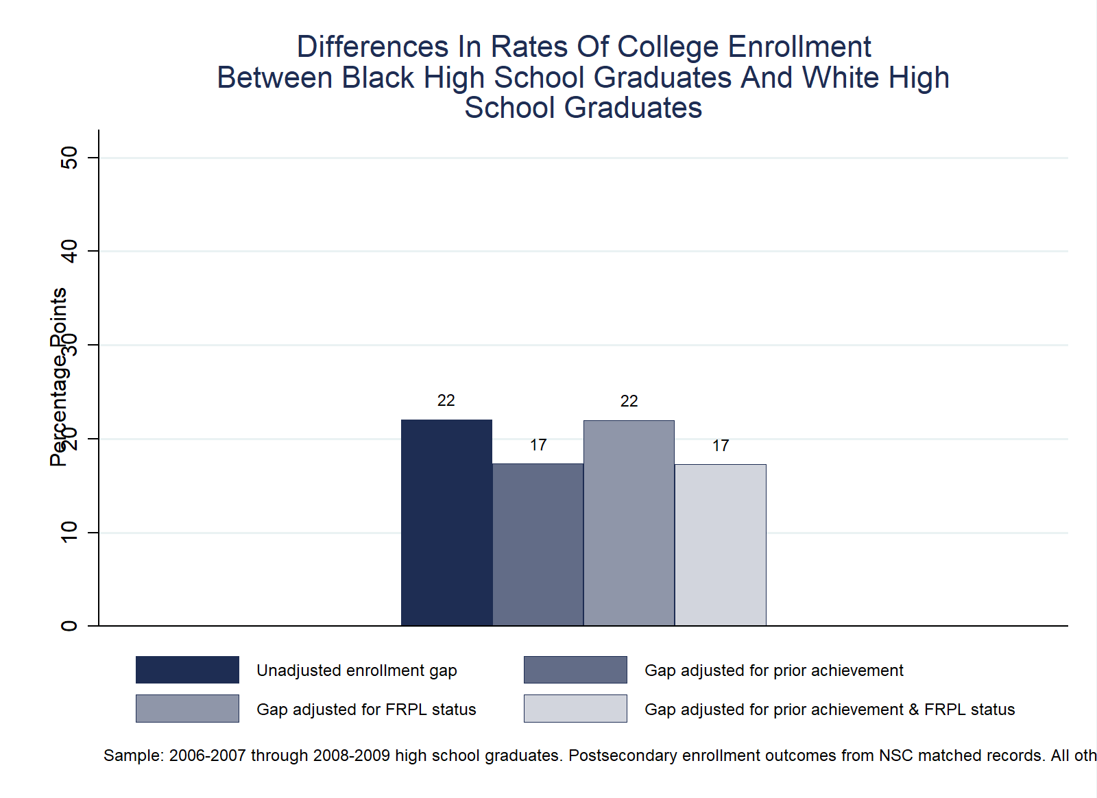
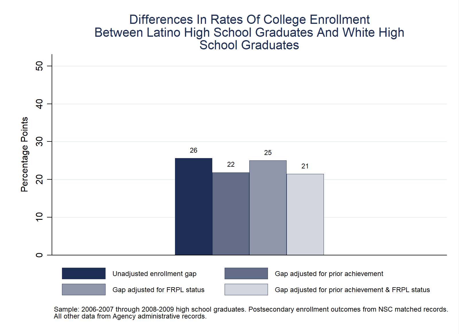
Purpose: This Strategic Performance Indicator explores gaps in college enrollment rates by ethnicity, before and after accounting for differences in prior academic achievement, socioeconomic status, and both of these background characteristics. While the analysis evaluates separately the college enrollment gaps between Black and White students and between Latino and White students, it can be modified to focus on the gap between any two races or ethnicities.
Required Analysis File Variables:
sidchrt_gradlast_hs_coderace_ethnicitytest_math_8frpl_everenrl_1oct_grad_yr1_anyAnalysis-Specific Sample Restrictions:
Ask Yourself
Analytic Technique: Calculate the difference between the proportion of Black (or Latino) high school graduates and the proportion of White high school graduates who enrolled in college—in raw terms and after accounting for 8th grade test scores, for eligibility for Free or Reduced Price Lunch (FRPL), and for both of these characteristics.
// Gaps in Rates of College Enrollment Between Latino and White Graduates

// Step 1: Load the college-going analysis file into Stata
use "$data/college_going_analysis", clear

// Step 2: Keep students in high school graduation cohorts you can observe enrolling in college the fall after graduation AND have non-missing eighth grade test scores AND non-missing FRPL status
local chrt_grad_begin = ${chrt_grad_begin}
local chrt_grad_end = ${chrt_grad_end}
keep if (chrt_grad >= `chrt_grad_begin' & chrt_grad <= `chrt_grad_end')
keep if frpl_ever != . | test_math_8 != .

// Step 3: Include only black, Latino, and white students
keep if race_ethnicity==1 | race_ethnicity == 3 | race_ethnicity == 5
gen afam = (race_ethnicity == 1)
gen hisp = (race_ethnicity == 3)
gen white = (race_ethnicity == 5)

// Step 4: Estimate the unadjusted and adjusted differences in college enrollment between Latino and white students and between black and white students.

// 1. Create a unique codeentifier for each cohort at each high school, so that we can cluster the standard errors at the cohort/high school level
egen cluster_var = concat(chrt_grad last_hs_code)

// 2. Fit 4 separate regression models with and without control variables, and save the coefficients associated with each race.
// 2A. Estimate unadjusted enrollment gap
reg enrl_1oct_grad_yr1_any afam hisp, robust cluster(cluster_var)
gen afam_unadj = _b[afam]
gen hisp_unadj = _b[hisp]

// 2B. Estimate enrollment gap adjusting for prior achievement
reg enrl_1oct_grad_yr1_any afam hisp test_math_8, robust cluster(cluster_var)
gen afam_adj_prior_ach = _b[afam]
gen hisp_adj_prior_ach = _b[hisp]

// 2C. Estimate enrollment gap adjusting for FRPL status
reg enrl_1oct_grad_yr1_any afam hisp frpl_ever, robust cluster(cluster_var)
gen afam_adj_frpl = _b[afam]
gen hisp_adj_frpl = _b[hisp]

// 2D. Estimate enrollment gap adjusting for prior achievement and FRPL status
reg enrl_1oct_grad_yr1_any afam hisp frpl_ever test_math_8, robust cluster(cluster_var)
gen afam_adj_prior_frpl = _b[afam]
gen hisp_adj_prior_frpl = _b[hisp]

//3. Transform the regression coefficients estimated in Step 4.2 to be displayed in positive % terms
foreach race in afam hisp {
    replace `race'_unadj = (0 - `race'_unadj) * 100
    replace `race'_adj_prior_ach = (0 - `race'_adj_prior_ach) * 100
    replace `race'_adj_frpl = (0 - `race'_adj_frpl) * 100
    replace `race'_adj_prior_frpl = (0 - `race'_adj_prior_frpl) * 100
}

// Step 5: Retain a data file containing only the regression coefficients
keep afam_* hisp_*
duplicates drop

// Step 6: Prepare to graph the results
// Generate a cohort label to be used in the footnote for the graph
local temp_begin = `chrt_grad_begin'-1
local temp_end = `chrt_grad_end'-1
if `chrt_grad_begin'==`chrt_grad_end' {
    local chrt_label "`temp_begin'-`chrt_grad_begin'"
}
else {
    local chrt_label "`temp_begin'-`chrt_grad_begin' through `temp_end'-`chrt_grad_end'"
}

// Step 7: Graph the results
// 1. Graph results for black and white students
#delimit ;
graph bar afam_unadj afam_adj_prior_ach afam_adj_frpl afam_adj_prior_frpl,
    legend(row(2) size(vsmall) region(lcolor(white))
    label(1 "Unadjusted enrollment gap")
    label(2 "Gap adjusted for prior achievement")
    label(3 "Gap adjusted for FRPL status")
    label(4 "Gap adjusted for prior achievement & FRPL status"))
outergap(300)
blabel(bar, format(%9.0f) size(vsmall))
    bar(1, fcolor(dknavy) lcolor(dknavy) fi(inten100))
    bar(2, fcolor(dknavy) lcolor(dknavy) fi(inten70))
    bar(3, fcolor(dknavy) lcolor(dknavy) fi(inten50))
    bar(4, fcolor(dknavy) lcolor(dknavy) fi(inten20))
    title("Differences In Rates Of College Enrollment"
    "Between Black High School Graduates And White High"
    "School Graduates", size(med))
    ytitle("Percentage Points", margin(2 2 0 0) size(small))
    yscale(range(0(10)50)) ylabel(0(10)50, labsize(small))
    graphregion(color(white) fcolor(white) lcolor(white))
    plotregion(color(white) fcolor(white) lcolor(white))
note("Sample: `chrt_label' high school graduates. Postsecondary enrollment outcomes from NSC matched records. All other data from ${agency_name} administrative records.", size(vsmall));
#delimit cr

graph export "figures/D6a_Col_Enrl_Gap_Black.png", replace width(1600) height(1200)

#delimit ;
graph bar hisp_unadj hisp_adj_prior_ach hisp_adj_frpl hisp_adj_prior_frpl,
    legend(row(2) size(vsmall) region(lcolor(white))
    label(1 "Unadjusted enrollment gap")
    label(2 "Gap adjusted for prior achievement")
    label(3 "Gap adjusted for FRPL status")
    label(4 "Gap adjusted for prior achievement & FRPL status"))
    outergap(300)
blabel(bar, format(%9.0f) size(vsmall))
    bar(1, fcolor(dknavy) lcolor(dknavy) fi(inten100))
    bar(2, fcolor(dknavy) lcolor(dknavy) fi(inten70))
    bar(3, fcolor(dknavy) lcolor(dknavy) fi(inten50))
    bar(4, fcolor(dknavy) lcolor(dknavy) fi(inten20))
    title("Differences In Rates Of College Enrollment"
    "Between Latino High School Graduates And White High"
    "School Graduates", size(med))
    ytitle("Percentage Points", margin(2 2 0 0) size(small))
    yscale(range(0(10)50)) ylabel(0(10)50, labsize(small))
    graphregion(color(white) fcolor(white) lcolor(white))
    plotregion(color(white) fcolor(white) lcolor(white))
note("Sample: `chrt_label' high school graduates. Postsecondary enrollment outcomes from NSC matched records." "All other data from ${agency_name} administrative records.", size(vsmall));
#delimit cr

graph export "figures/D6b_Col_Enrl_Gap_Latino.png", replace width(1600) height(1200)
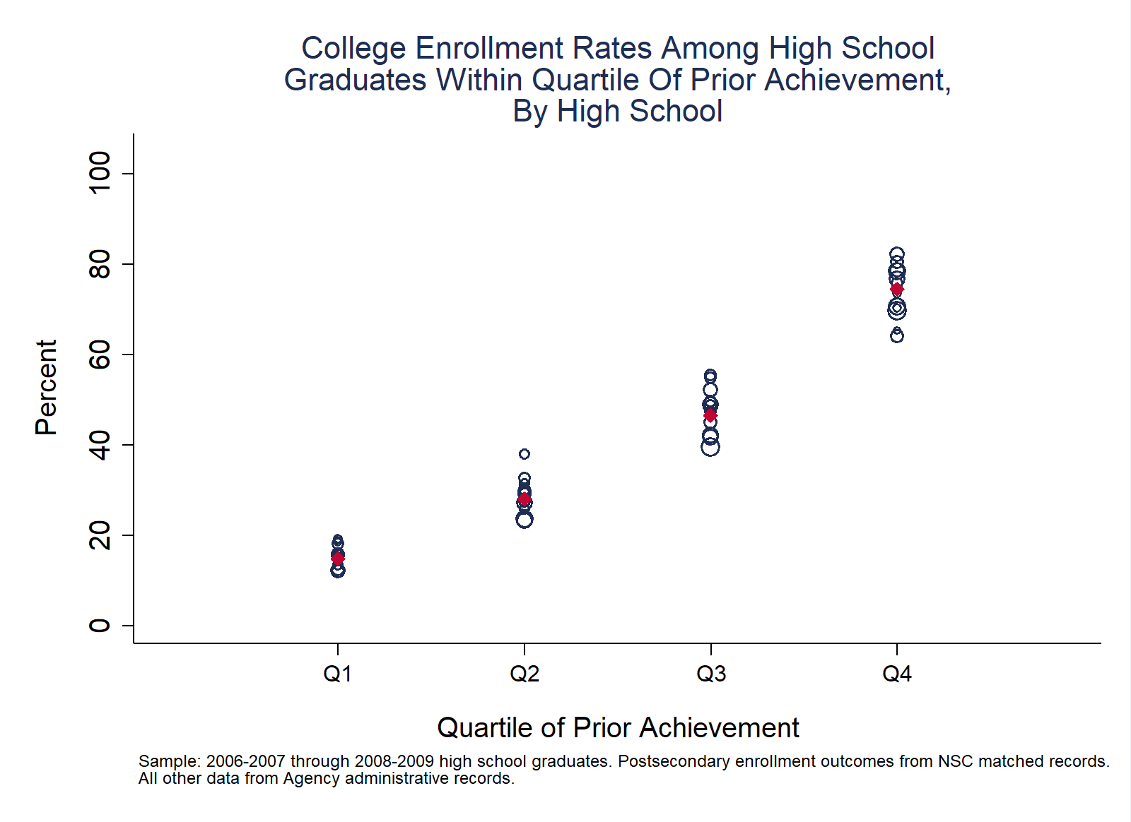
Purpose: This SPI highlights the variation in college-going rates across high schools when students with similar prior achievement are compared. To conduct these comparisons, we first sort all incoming ninth-graders into quartiles based on their 8th grade test scores. We then examine college-going rates by high school among graduates within each of these quartiles.
Required Analysis File Variables:
sidchrt_gradlast_hs_namehs_diplomaqrt_8_math_stdenrl_1oct_grad_yr1_anyAnalysis-Specific Sample Restrictions:
Ask Yourself
Analytic Technique: Calculate the share of students in each 8th grade test score quartile at each high school who enroll in college seamlessly after high school graduation.
// College Enrollment Rates by 8th Grade Achievement Quartile Bubbles

// Step 1: Load the college-going analysis file into Stata
use "$data/college_going_analysis", clear

// Step 2: Keep students in high school graduation cohorts you can observe enrolling in college the fall after graduation AND have non-missing eighth grade test scores
local chrt_grad_begin = ${chrt_grad_begin}
local chrt_grad_end = ${chrt_grad_end}
keep if (chrt_grad >= `chrt_grad_begin' & chrt_grad <= `chrt_grad_end')
keep if qrt_8_math != .

// Step 3: Create agency- and school-level average outcomes for each quartile
// 1. Calculate the mean of each outcome variable by high school
collapse (sum) enrl_1oct_grad_yr1_any hs_diploma, by(last_hs_name qrt_8_math)
gen pct_enrl = enrl_1oct_grad_yr1_any / hs_diploma * 100
// 2. Calculate the mean of each outcome variable for the agency as a whole
egen num = sum(enrl_1oct_grad_yr1_any), by(qrt_8_math)
egen denom = sum(hs_diploma), by(qrt_8_math)
gen agency_avg = num / denom * 100
drop num denom

// Step 4: Create a variable to identify the test score quartile
gen agency_quartile_code = .
forvalues qrt = 1(1)4 {
    local qrt_plot = `qrt' * 2
    replace agency_quartile_code = 1.`qrt_plot' if qrt_8_math == `qrt'
}

// Step 5: Prepare to graph the results
// Generate a cohort label to be used in the footnote for the graph
local temp_begin = `chrt_grad_begin'-1
local temp_end = `chrt_grad_end'-1
if `chrt_grad_begin'==`chrt_grad_end' {
    local chrt_label "`temp_begin'-`chrt_grad_begin'"
}
else {
    local chrt_label "`temp_begin'-`chrt_grad_begin' through `temp_end'-`chrt_grad_end'"
}

// Step 6: Graph the results
#delimit ;
graph twoway scatter pct_enrl agency_quartile_code [aweight = hs_diploma],
    msymbol(Oh) msize(vsmall) mcolor(dknavy) ||
scatter agency_avg agency_quartile_code,
    mcolor(cranberry) msymbol(D) msize(small)
title("College Enrollment Rates Among High School"
"Graduates Within Quartile Of Prior Achievement,"
"By High School", size(med))
    xscale(range(1 2)) yscale(range(0 105)) ylabel(0 20 40 60 80 100)
    xlabel(1.2 "Q1" 1.4 "Q2" 1.6 "Q3" 1.8 "Q4", labsize(small))
    xtitle(" " "Quartile of Prior Achievement") ytitle("Percent" " ")
    ylabel(,nogrid) legend(off)
graphregion(color(white) fcolor(white) lcolor(white))
plotregion(color(white) fcolor(white) lcolor(white))
note("Sample: `chrt_label' high school graduates. Postsecondary enrollment outcomes from NSC matched records."
"All other data from ${agency_name} administrative records.", size(vsmall));
#delimit cr

graph export "figures/D7_Col_Enrl_by_Eighth_Qrt_Bubbles.png", replace width(1600) height(1200)
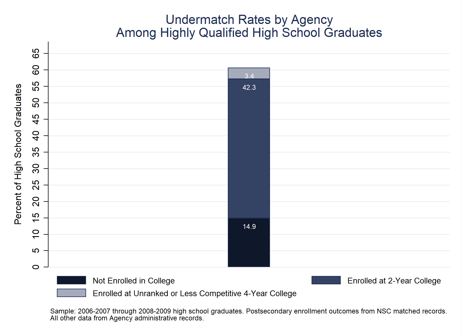
Purpose: This Strategic Performance Indicator examines the prevalence of “undermatch” in the agency—that is, the extent to which high school graduates with strong academic records pursue enrollment in colleges and universities less selective than those for which they are likely qualified. The SPI does so by illustrating the rates at which highly qualified graduates are enrolling at 2-year colleges, less competitive 4-year colleges, or forgoing college altogether, instead of pursuing selective colleges that may provide a better academic and social fit for these students’ potential, ambition, and preparation.
Required Analysis File Variables:
sidchrt_gradhighly_qualifiedfirst_college_opeid_4yrenrl_1oct_grad_yr1_anyenrl_1oct_grad_yr1_4yrenrl_1oct_grad_yr1_2yrAnalysis-Specific Sample Restrictions:
Ask Yourself
// Undermatch Rates Among Highly Qualified High School Graduates

// Step 1: Load the post-sec analysis file into Stata
use "$data/college_going_analysis", clear

// Step 2: Keep students in high school graduation cohorts you can observe enrolling in college the fall after graduation AND are highly qualified
local chrt_grad_begin = ${chrt_grad_begin}
local chrt_grad_end = ${chrt_grad_end}
keep if (chrt_grad >= `chrt_grad_begin' & chrt_grad <= `chrt_grad_end')
keep if highly_qualified == 1

// Step 3: Create college enrollment indicator variables for each college selectivity level. This script assumes that there are 5 levels of selectivity, as in Barron's College Rankings: Most Competitive (1), Highly Competitive (2), Very Competitive (3), Competitive (4), Least Competitive (5), as well as a category for colleges without assigned selectivity (assumed to be not competitive).
//1. Create college enrollment dummy variables for each of the five selectivity levels
forvalues i = 1/5 {
    gen enrl_1oct_grad_yr1_4yr_`i' = (enrl_1oct_grad_yr1_4yr == 1 & rank == `i')
}

//2. Create a college enrollment dummy variable for colleges that are not ranked
gen enrl_1oct_grad_4yr_nr = (enrl_1oct_grad_yr1_4yr == 1 & (rank == 6 | rank ==. ))

//3. Rename and label the college enrollment variables with clear labels
rename enrl_1oct_grad_yr1_4yr_1 enrl_1oct_grad_4yr_mc
rename enrl_1oct_grad_yr1_4yr_2 enrl_1oct_grad_4yr_hc
rename enrl_1oct_grad_yr1_4yr_3 enrl_1oct_grad_4yr_vc
rename enrl_1oct_grad_yr1_4yr_4 enrl_1oct_grad_4yr_c
rename enrl_1oct_grad_yr1_4yr_5 enrl_1oct_grad_4yr_lc

label var enrl_1oct_grad_4yr_mc "Enrolled at Most Competitive College Fall After HS Grad"
label var enrl_1oct_grad_4yr_hc "Enrolled at Highly Competitive College Fall After HS Grad"
label var enrl_1oct_grad_4yr_vc "Enrolled at Very Competitive College Fall After HS Grad"
label var enrl_1oct_grad_4yr_c "Enrolled at Competitive College Fall After HS Grad"
label var enrl_1oct_grad_4yr_lc "Enrolled at Least Competitive College Fall After HS Grad"
label var enrl_1oct_grad_4yr_nr "Enrolled at Non-Competitive College Fall After HS Grad"

//4. Check to make sure that each student who appears enrolled in college as of the first fall after high school graduation is associated with one and only one college selectivity level
assert enrl_1oct_grad_4yr_mc + enrl_1oct_grad_4yr_hc + enrl_1oct_grad_4yr_vc + enrl_1oct_grad_4yr_c + enrl_1oct_grad_4yr_lc + enrl_1oct_grad_4yr_nr == 1 if enrl_1oct_grad_yr1_4yr == 1

// Step 4: Create undermatch outcomes
//1. Not enrolled in college
gen no_college = (enrl_1oct_grad_yr1_any == 0)

//2. Enrolled in a 2-year college
gen enrl_2yr = (enrl_1oct_grad_yr1_2yr == 1)

//3. Enrolled in a least competitive 4-year college or a 4-year college without an assigned selectivity
gen enrl_4yr_under = (enrl_1oct_grad_4yr_nr == 1)
replace enrl_4yr_under = 1 if enrl_1oct_grad_4yr_lc == 1

//4. Enrolled in a 4-year college with a selectivity rating of Competitive, Very Competitive, Most Competitive, or Highly Competitive
gen enrl_4yr_match = (enrl_1oct_grad_4yr_c == 1 | enrl_1oct_grad_4yr_vc == 1 | enrl_1oct_grad_4yr_hc == 1 | enrl_1oct_grad_4yr_mc == 1)

//5. Check to make sure that each student is associated one and only one undermatch outcome
// assert no_college + enrl_2yr + enrl_4yr_under + enrl_4yr_match == 1

// Step 5: Create agency-average undermatch outcomes and transform them into % terms
collapse (mean) no_college enrl_2yr enrl_4yr_under enrl_4yr_match (count) N = sid
foreach v of varlist no_college enrl_2yr enrl_4yr_under enrl_4yr_match {
    replace `v' = round(`v' * 100, 0.1)
}

// Step 6: Prepare to graph the results
// Generate a cohort label to be used in the footnote for the graph
local temp_begin = `chrt_grad_begin'-1
local temp_end = `chrt_grad_end'-1
if `chrt_grad_begin'==`chrt_grad_end' {
    local chrt_label "`temp_begin'-`chrt_grad_begin'"
}
else {
    local chrt_label "`temp_begin'-`chrt_grad_begin' through `temp_end'-`chrt_grad_end'"
}

// Step 7: Graph the results
#delimit ;
graph bar no_college enrl_2yr enrl_4yr_under, stack
    blabel(bar, format(%9.1f) size(2.05) position(inside) color(white))
    bar(1, fcolor(dknavy) lcolor(dknavy) finten(200) lwidth(thin))
    bar(2, fcolor(dknavy) lcolor(dknavy) finten(90) lwidth(thin))
    bar(3, fcolor(dknavy) lcolor(dknavy) finten(40) lwidth(thin))
    yscale(range(0(5)65)) outergap(400)
    ylabel(0(5)65, labsize(small))
title("Undermatch Rates by Agency"
    "Among Highly Qualified High School Graduates", size(med))
    ytitle("Percent of High School Graduates" " ", size(small))
legend(region(lcolor(white))
    label(1 "Not Enrolled in College")
    label(2 "Enrolled at 2-Year College")
    label(3 "Enrolled at Unranked or Less Competitive 4-Year College")
    symxsize(*.7) symysize(*.7) size(*.7))
graphregion(color(white) fcolor(white) lcolor(white))
plotregion(color(white) fcolor(white) lcolor(white))
note("Sample: `chrt_label' high school graduates. Postsecondary enrollment outcomes from NSC matched records."
"All other data from ${agency_name} administrative records.", size(vsmall)) ;
#delimit cr

graph export "figures/D8_Undermatching_HiQualified.png", replace width(1600) height(1200)