
In this guide you will be able to visualize high school graduation rates by high school, student achievement level before high school, student race/ethnicity, on-track status after ninth-grade.
The College-Going Pathways series is a set of guides, code, and sample data about policy-relevant college-going topics. Browse this and other guides in the series for ideas about ways to investigate student pathways through high school and college. Each guide includes several analyses in the form of charts together with Stata analysis and graphing code to generate each chart.
Once you’ve identified analyses that you want to try to replicate or modify, click the “Download” buttons to download Stata code and sample data. You can make changes to the charts using the code and sample data, or modify the code to work with your own data. If you’re familiar with Github, you can click “Go to Repository” and clone the entire College-Going Pathways repository to your own computer.
The data visualizations in the College-Going Pathways series use a synthetically generated college-going analysis sample data file which has one record per student. Each high school student is assigned to a ninth-grade cohort, and each student record includes demographic and program participation information, annual GPA and on-track status, high school graduation outcomes, and college enrollment information. The Connect guide (coming soon) will provide guidance and example code which will help you build a college-going analysis file using data from your own school system.
High school graduation is a critical step to higher education. Understanding trends and variations in high school completion rates across schools and student subgroups is essential. These analyses reveal the extent to which high schools may differentially influence student trajectories towards high school completion. After identifying these high schools, you may conduct deeper analyses on your own to explore what drives these outcomes.
One of the most important decisions in running each analysis is defining the sample. Each analysis corresponds to a different part of the education pipeline and as a result requires different cohorts of students.
If you are using the synthetic data we have provided, the sample restrictions have been predefined and are included below. If you run this code using your own agency data, change the sample restrictions based on your data. Note that you will have to run these sample restrictions at the beginning of your do file so they will feed into the rest of your code.
// Sample Restrictions

// Agency name
global agency_name "Agency"

// Ninth grade cohorts you can observe persisting to the second year of college
global chrt_ninth_begin_persist_yr2 = 2004
global chrt_ninth_end_persist_yr2 = 2006

// Ninth grade cohorts you can observe graduating high school on time
global chrt_ninth_begin_grad = 2004
global chrt_ninth_end_grad = 2006

// Ninth grade cohorts you can observe graduating high school one year late
global chrt_ninth_begin_grad_late = 2004
global chrt_ninth_end_grad_late = 2006

// High school graduation cohorts you can observe enrolling in college the fall after graduation
global chrt_grad_begin = 2007
global chrt_grad_end = 2009

// High school graduation cohorts you can observe enrolling in college two years after hs graduation
global chrt_grad_begin_delayed = 2007
global chrt_grad_end_delayed = 2009
Based on the sample data, you will have three cohorts (sometimes only two) for analysis. If you are using your own agency data, you may decide to aggregate results for more or fewer cohorts to report your results. This decision depends on 1) how much historical data you have available and 2) what balance to strike between reliability and averaging away information on recent trends. We suggest you average results for the last three cohorts to take advantage of larger sample sizes and improve reliability. However, if you have data for more than three cohorts, you may decide to not average data out for fear of losing information about trends and recent changes in your agency.
This guide is an open-source document hosted on Github and generated using the Stata Webdoc package. We welcome feedback, corrections, additions, and updates. Please visit the OpenSDP college-going pathways repository to read our contributor guidelines.
Purpose: This analysis explores variation in high school completion rates across high schools in the system for both on-time and late high school graduates.
Required Analysis File Variables:
sidchrt_ninthhs_diplomaontime_gradlate_gradfirst_hs_codefirst_hs_nameAnalysis-Specific Sample Restrictions: Keep students in ninth grade cohorts you can observe graduating high school one year late
Ask Yourself
Does the ordering of high school completion rates coincide with beliefs key stakeholders have about these high schools?
Which high schools have the highest and lowest completion rates? Do you know why?
Analytic Technique: Calculate the proportion of students who complete high school by school.
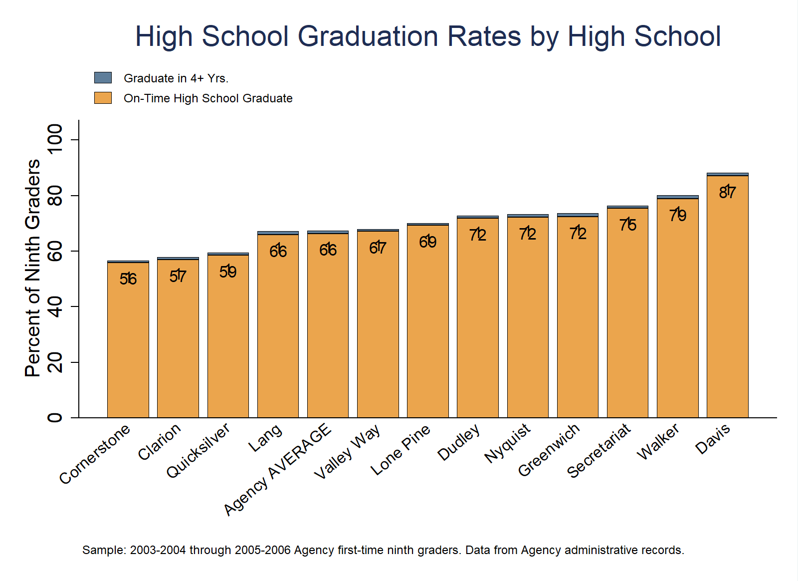
// High School Completion Rates By School

// Step 1: Load the college-going analysis file into Stata
use "$data/college_going_analysis", clear

// Step 2: Keep students in ninth grade cohorts you can observe graduating high school one year late
local chrt_ninth_begin = ${chrt_ninth_begin_grad_late}
local chrt_ninth_end = ${chrt_ninth_end_grad_late}
keep if (chrt_ninth >= `chrt_ninth_begin' & chrt_ninth <= `chrt_ninth_end')

// Step 3: Obtain the agency-level high school graduation rates.
preserve
    collapse (mean) ontime_grad late_grad (count) N = sid
    tempfile agency_level
    save `agency_level'
restore

// Step 4: Obtain the school-level high school graduation rates and append the agency average
collapse (mean) ontime_grad late_grad (count) N = sid, by(first_hs_name first_hs_code)
append using `agency_level'

// Step 5: Provide a hs name label for the appended agency average and shorten hs name
replace first_hs_code = 0 if first_hs_code == .
replace first_hs_name = "${agency_name} AVERAGE" if mi(first_hs_name)
replace first_hs_name = subinstr(first_hs_name, " High School", "", .)

// Step 6: Multiply the average of each outcome by 100 for graphical representation of the rates
foreach var of varlist ontime_grad late_grad {
    replace `var' = `var' * 100
    format `var' %9.1f
}

// Step 7: Prepare to graph the results
// Generate a cohort label to be used in the footnote for the graph
local temp_begin = `chrt_ninth_begin'-1
local temp_end = `chrt_ninth_end'-1
if `chrt_ninth_begin'==`chrt_ninth_end' {
    local chrt_label "`temp_begin'-`chrt_ninth_begin'"
}
else {
    local chrt_label "`temp_begin'-`chrt_ninth_begin' through `temp_end'-`chrt_ninth_end'"
}

// Step 8: Graph the results
#delimit ;
graph bar (sum) ontime_grad late_grad, stack over(first_hs_name, label(angle(40)
    labsize(small)) gap(20) sort(ontime_grad))
    blabel(bar, position(inside) color(black) size(small) format(%8.0f))
    bar(1, fcolor(dkorange) fintensity(70) lcolor(black))
    bar(2, fcolor(navy) fintensity(70) lcolor(black))
legend(region(lcolor(white)) symxsize(3) symysize(2) rows(2) order(2 1) size(vsmall)
    position(11) label(1 "On-Time High School Graduate") label(2 "Graduate in 4+ Yrs."))
title("High School Graduation Rates by High School")
    ytitle("Percent of Ninth Graders") yscale(range(0(20)100)) ylabel(0(20)100, nogrid)
graphregion(color(white) fcolor(white) lcolor(white))
plotregion(color(white) fcolor(white) lcolor(white))
note(" " "Sample: `chrt_label' ${agency_name} first-time ninth graders. Data from ${agency_name} administrative records." , size(vsmall));
#delimit cr

graph export "figures/C1_HS_Grad_by_HS.png", replace width(1600) height(1200)
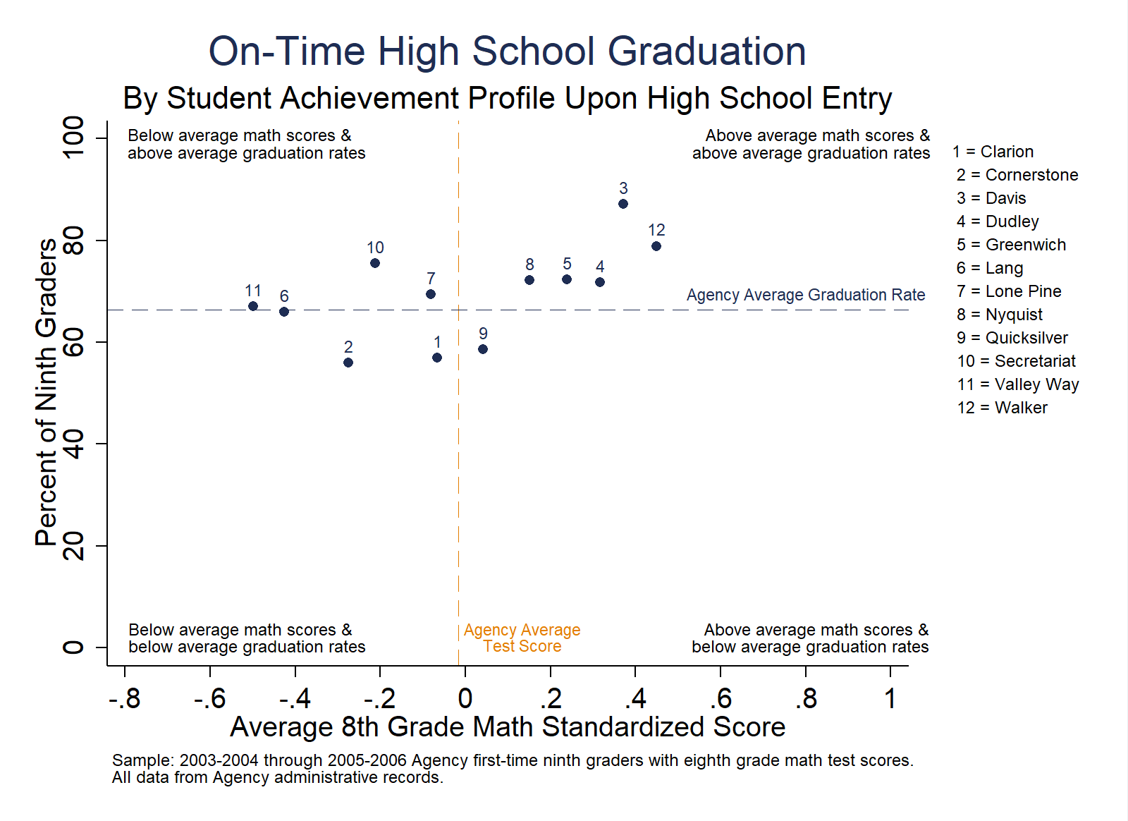
Purpose: This analysis examines the relationship between academic achievement at high school entry and high school completion rates. This analysis is useful to identify high schools that beat the odds. High schools with similar incoming student achievement profiles but different high school graduation rates.
Required Analysis File Variables:
sidchrt_ninthtest_math_8_stdhs_diplomafirst_hs_codefirst_hs_nameAnalysis-Specific Sample Restrictions:
Ask Yourself
What might explain differences in high school graduation rates for high schools with similar incoming achievement? What might explain differences in incoming achievement for high schools with similar graduation rates?
Possible Next Steps or Action Plans: If substantial variation exists after controlling for average student achievement at high school entry, think about how to share this information across schools. To explore mechanisms that drive school-level differences in high school completion rates, replicate this analysis where the x-axis is a middle school at-risk index (e.g. an index that accounts for whether students failed a core class, were chronically absent, and other information predictive of student achievement in high school) in place of 8th grade test scores.
Analytic Technique: Bivariate scatterplot of school-level average student test scores and high school completion rates.
// High School Completion Rates by Average 8th Grade Achievement

// Step 1: Load the college-going analysis file into Stata.
use "$data/college_going_analysis", clear

// Step 2: Keep students in ninth grade cohorts you can observe graduating high school AND have non-missing eighth grade math scores.
local chrt_ninth_begin = ${chrt_ninth_begin_grad}
local chrt_ninth_end = ${chrt_ninth_end_grad}
keep if (chrt_ninth >= `chrt_ninth_begin' & chrt_ninth <= `chrt_ninth_end') & !mi(test_math_8_std)

// Step 3: Obtain agency-level high school completion rate and prior achievement score along with the position of their labels.
summ ontime_grad
local agency_mean_grad = `r(mean)'*100
local agency_mean_grad_label = `agency_mean_grad' + 3
summ test_math_8_std
local agency_mean_test = `r(mean)'
local agency_mean_test_label = `agency_mean_test' + 0.15

// Step 4: Obtain school-level high school completion and prior achievement rates
collapse (mean) test_math_8_std ontime_grad (count) N = sid, by(first_hs_code first_hs_name)
drop if N < 20

// Step 5: Multiply the high school completion rate by 100 for graphical representation of the rates,
replace ontime_grad = round((ontime_grad * 100), .1)

// Step 6: Shorten high school names and create a legend label for the graph
sort first_hs_name
replace first_hs_name = subinstr(first_hs_name, " High School", "", .)
gen hs_code_label = _n

levelsof first_hs_name, local(hs_names)
local count = 1
local legend_labels ""
foreach hs of local hs_names {
    local legend_labels `"`legend_labels' `count' = `hs'"' `" "'
    local ++count
}

// Step 7: Prepare to graph the results
// Generate a cohort label to be used in the footnote for the graph
local temp_begin = `chrt_ninth_begin'-1
local temp_end = `chrt_ninth_end'-1
if `chrt_ninth_begin'==`chrt_ninth_end' {
    local chrt_label "`temp_begin'-`chrt_ninth_begin'"
}
else {
    local chrt_label "`temp_begin'-`chrt_ninth_begin' through `temp_end'-`chrt_ninth_end'"
}

// Step 8: Graph the results
#delimit ;
twoway (scatter ontime_grad test_math_8_std, mlabel(hs_code_label) mlabsize(vsmall)
    mlabposition(12) mlabcolor(dknavy) mstyle(x) msize(small) mcolor(dknavy)),
title("On-Time High School Graduation")
    subtitle("By Student Achievement Profile Upon High School Entry")
    xtitle("Average 8th Grade Math Standardized Score", linegap(0.3))
    ytitle("Percent of Ninth Graders")
    xscale(range(-0.8(0.2)1)) xlabel(-0.8(0.2)1)
    yscale(range(0(20)100)) ylabel(0(20)100, nogrid)
    legend(on order(3) col(1) label(3 `"`legend_labels'"')
    region(color(none)) size(vsmall) position(2) ring(1) linegap(.75))
yline(`agency_mean_grad', lpattern(dash) lcolor(dknavy) lwidth(vvthin))
xline(`agency_mean_test', lpattern(dash) lcolor(dkorange) lwidth(vvthin))
text(`agency_mean_grad_label' .8 "${agency_name} Average Graduation Rate", size(2.0) color(dknavy))
text(2 `agency_mean_test_label' "${agency_name} Average" "Test Score", size(2.0) color(dkorange))
text(99 -.5 "Below average math scores &" "above average graduation rates",
    size(vsmall) justification(left))
text(99 0.8 "Above average math scores &" "above average graduation rates",
    size(vsmall) justification(right))
text(2 -0.5 "Below average math scores &" "below average graduation rates",
    size(vsmall) justification(left))
text(2 0.8 "Above average math scores &" "below average graduation rates",
    size(vsmall) justification(right))
graphregion(color(white) fcolor(white) lcolor(white))
plotregion(color(white) fcolor(white) lcolor(white))
note("Sample: `chrt_label' ${agency_name} first-time ninth graders with eighth grade math test scores." "All data from ${agency_name} administrative records.", size(vsmall));
#delimit cr

graph export "figures/C2_HS_Grad_by_Avg_Eighth.png", replace width(1600) height(1200)
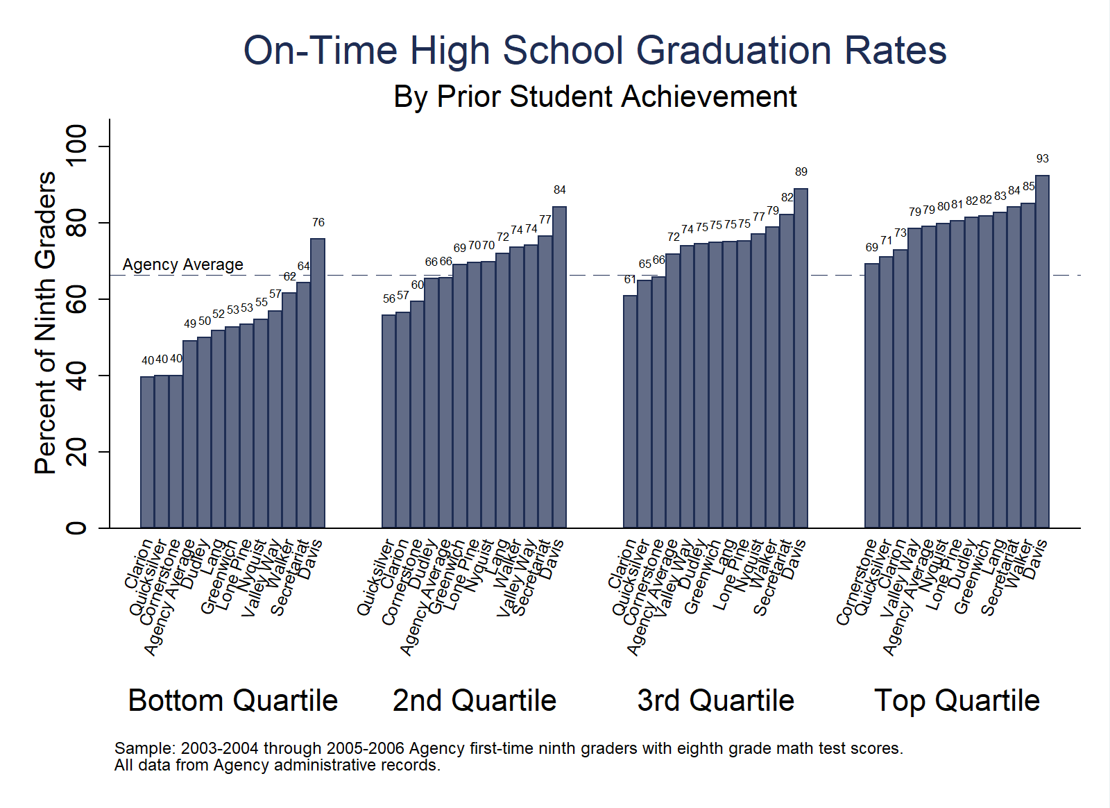
Purpose: This analysis examines variation in completion rates for high schools among students with 8th grade test scores in the same quartile. The analysis is useful to explore high school completion rates across schools with students in the same quartile or range of achievement. Each high school is repeated as a blue bar in each quartile.
Required Analysis File Variables:
sidchrt_ninthtest_math_8_stdhs_diplomafirst_hs_codefirst_hs_nameAnalysis-Specific Sample Restrictions:
Ask Yourself
Possible Next Steps or Action Plans: Highlight comparison schools to show variation across quartiles and explore reasons why students at different schools, but with similar academic profiles at high school entry, are more or less likely to graduate.
Analytic Technique: Calculate the proportion of students, by high school, who complete high school and an 8th grade test score quartile for each.
// High School Completion Rates by 8th Grade Achievement Quartiles

// Step 1: Load the college-going analysis file into Stata.
use "$data/college_going_analysis", clear

// Step 2: Keep students in ninth grade cohorts you can observe graduating high school AND have non-missing eighth grade math scores.
local chrt_ninth_begin = ${chrt_ninth_begin_grad}
local chrt_ninth_end = ${chrt_ninth_end_grad}
keep if (chrt_ninth >= `chrt_ninth_begin' & chrt_ninth <= `chrt_ninth_end') & !mi(test_math_8)

// Step 3: Obtain the overall agency-level high school graduation rate along with the position of its label.
summ ontime_grad
local agency_mean = `r(mean)'*100
local agency_mean_label = `agency_mean'+3

// Step 4: Obtain the agency-level high school graduation rates by test score quartile.
preserve
    collapse (mean) ontime_grad (count) N = sid, by(qrt_8_math)
    tempfile agency_level
    save `agency_level'
restore

// Step 5: Obtain school-level high school graduation rates by test score quartile and append the agency-level graduation rates by quartile
collapse (mean) ontime_grad (count) N = sid, by(first_hs_code first_hs_name qrt_8_math)
append using `agency_level'

// Step 6: Shorten high school names and drop any high schools with fewer than 20 students
replace first_hs_code = 0 if first_hs_code == .
replace first_hs_name = "${agency_name} Average" if mi(first_hs_name)
replace first_hs_name = subinstr(first_hs_name, " High School", "", .)
drop if N < 20

// Step 7: Multiply the high school completion rate by 100 for graphical representation of the rates
replace ontime_grad = round((ontime_grad * 100), .1)

// Step 8: Create a variable to sort schools within each test score quartile in ascending order
sort qrt_8_math ontime_grad
gen rank = _n

// Step 9: Prepare to graph the results
// Generate a cohort label to be used in the footnote for the graph
local temp_begin = `chrt_ninth_begin'-1
local temp_end = `chrt_ninth_end'-1
if `chrt_ninth_begin'==`chrt_ninth_end' {
    local chrt_label "`temp_begin'-`chrt_ninth_begin'"
}
else {
    local chrt_label "`temp_begin'-`chrt_ninth_begin' through `temp_end'-`chrt_ninth_end'"
}

// Step 10: Graph the results
#delimit ;
graph bar ontime_grad, over(first_hs_name, sort(rank) gap(0) label(angle(70) labsize(vsmall)))
    over(qrt_8_math, relabel(1 "Bottom Quartile" 2 "2nd Quartile" 3 "3rd Quartile" 4 "Top Quartile") gap(400))
    bar(1, fcolor(dknavy) finten(70) lcolor(dknavy) lwidth(thin))
    blabel(bar, format(%8.0f) size(1.5))
    yscale(range(0(20)100)) ylabel(0(20)100, nogrid) legend(off)
title("On-Time High School Graduation Rates")
    subtitle("By Prior Student Achievement", size(msmall))
    ytitle("Percent of Ninth Graders")
    yline(`agency_mean', lpattern(dash) lwidth(vvthin) lcolor(dknavy))
text(`agency_mean_label' 5 "${agency_name} Average", size(vsmall))
graphregion(color(white) fcolor(white) lcolor(white))
plotregion(color(white) fcolor(white) lcolor(white))
note(" " "Sample: `chrt_label' ${agency_name} first-time ninth graders with eighth grade math test scores." "All data from ${agency_name} administrative records.", size(vsmall));
#delimit cr

graph export "figures/C3_HS_Grad_by_Eighth_Qrt.png", replace width(1600) height(1200)
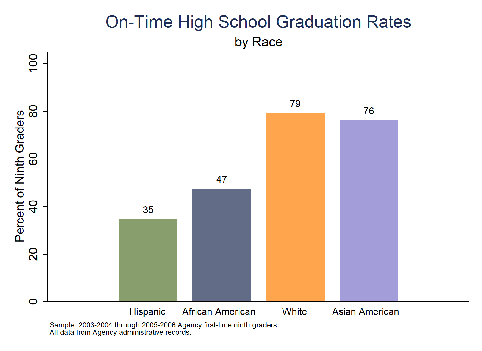
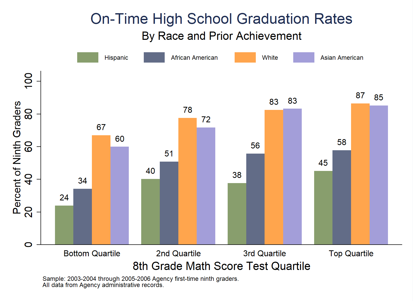
Purpose: This analysis displays an overall graduation gap by race, and examines the extent to which this gap is explained by average differences in academic achievement between racial sub-groups at high school entry. The analysis is useful to diagnose whether racial gaps in high school result from persistent academic achievement gaps that emerge in early grades, or if other factors unique to the high school experience drive high school completion rate differences by race.
Required Analysis File Variables:
sidchrt_ninthtest_math_8_stdhs_diplomafirst_hs_codefirst_hs_nameAnalysis-Specific Sample Restrictions:
Ask Yourself
Possible Next Steps or Action Plans: Repeat analyses for only students that qualify for free or reduced price lunch (FRPL) to explore if racial gaps are better explained by disparities in prior academic achievement and family socioeconomic status.
Analytic Technique: Calculate the proportion of students who complete high school by race/ethnicity overall, and by race/ethnicity and 8th grade test score quartile.
// Racial Gaps in Completion Overall and by 8th Grade Achievement Quartiles

// Step 1: Load the college-going analysis file into Stata
use "$data/college_going_analysis", clear

// Step 2: Keep students in ninth grade cohorts you can observe graduating high school AND have non-missing eighth grade math scores
local chrt_ninth_begin = ${chrt_ninth_begin_grad}
local chrt_ninth_end = ${chrt_ninth_end_grad}
keep if (chrt_ninth >= `chrt_ninth_begin' & chrt_ninth <= `chrt_ninth_end') & !mi(test_math_8)

// Step 3: Obtain the average on-time high school completion rate by race/ethnicity; you will restore in step 8
preserve
    collapse (mean) ontime_grad (count) N=sid, by(race_ethnicity)

// Step 4: Multiply the high school completion rate by 100 for graphical representation of the rates
    replace ontime_grad = (ontime_grad * 100)

// Step 5: Reshape the data wide so that each race is associated with the outcome variable
    gen id = _n
    reshape wide ontime_grad, i(id) j(race_ethnicity)

// Step 6: Prepare to graph the results
// Generate a cohort label to be used in the footnote for the graph
local temp_begin = `chrt_ninth_begin'-1
local temp_end = `chrt_ninth_end'-1
if `chrt_ninth_begin'==`chrt_ninth_end' {
    local chrt_label "`temp_begin'-`chrt_ninth_begin'"
}
else {
    local chrt_label "`temp_begin'-`chrt_ninth_begin' through `temp_end'-`chrt_ninth_end'"
}

// Step 7: Graph the results (1/2)
#delimit ;
graph bar ontime_grad3 ontime_grad1 ontime_grad5 ontime_grad2,
    bargap(25) outergap(100)
    bar(1, fcolor(forest_green*.7) lcolor(forest_green*.7))
    bar(2, fcolor(dknavy*.7) lcolor(dknavy*.7))
    bar(3, fcolor(orange*.7) lcolor(orange*.7))
    bar(4, fcolor(lavender*.85) lcolor(lavender*.85))
    blabel(bar, size(small) format(%8.0f))
text(-4 22 "Hispanic", size(small))
text(-4 40 "African American", size(small))
text(-4 59 "White", size(small))
text(-4 77 "Asian American", size(small))
title("On-Time High School Graduation Rates")
    subtitle("by Race")
    ytitle("Percent of Ninth Graders")
    yscale(range(0(20)100))
    ylabel(0(20)100, nogrid)
legend(off)
graphregion(color(white) fcolor(white) lcolor(white))
plotregion(color(white) fcolor(white) lcolor(white))
note(" " " " "Sample: `chrt_label' ${agency_name} first-time ninth graders." "All data from ${agency_name} administrative records.", size(vsmall));
#delimit cr

graph export "figures/C4a_HS_Grad_by_Race.png", replace width(1600) height(1200)

// Step 8: Restore the data and repeat steps 3-6 to obtain completion rates by race/ethnicity and eighth grade test score quartiles
restore
collapse (mean) ontime_grad (count) N=sid, by(race_ethnicity qrt_8_math)
replace ontime_grad = (ontime_grad * 100)
reshape wide ontime_grad, i(qrt_8_math N) j(race_ethnicity)

// Step 9: Graph the results (2/2)
#delimit ;
graph bar ontime_grad3 ontime_grad1 ontime_grad5 ontime_grad2, over(qrt_8_math,
    relabel(1 "Bottom Quartile" 2 "2nd Quartile" 3 "3rd Quartile" 4 "Top Quartile") label(labsize(small)))
    bar(1, fcolor(forest_green*.7) lcolor(forest_green*.7)) bar(2, fcolor(dknavy*.7) lcolor(dknavy*.7))
    bar(3, fcolor(orange*.7) lcolor(orange*.7)) bar(4, fcolor(lavender*.85) lcolor(lavender*.85))
    blabel(bar, format(%8.0f))
title("On-Time High School Graduation Rates")
    subtitle("By Race and Prior Achievement")
    b1title("8th Grade Math Score Test Quartile")
    ytitle("Percent of Ninth Graders") yscale(range(0(20)100)) ylabel(0(20)100, nogrid)
legend(order(1 2 3 4) row(1) label(1 "Hispanic")
    label(2 "African American") label(3 "White") label(4 "Asian American") size(vsmall)
    symxsize(7) position(inside) ring(1) region(lstyle(none)
    lcolor(none) color(none)))
graphregion(color(white) fcolor(white) lcolor(white))
plotregion(color(white) fcolor(white) lcolor(white))
note("Sample: `chrt_label' ${agency_name} first-time ninth graders." "All data from ${agency_name} administrative records.", size(vsmall));
#delimit cr
graph export "figures/C4b_HS_Grad_by_Race_by_Eighth_Qrt.png", replace width(1600) height(1200)
Purpose: This analysis explores how strongly student performance in ninth grade predicts high school graduation three years later. Building upon our analysis of the relationship between student performance in ninth and tenth grade, the analysis assesses the utility of using course-level performance data early in students’ high school careers to assess risk of non-completion, and target students in need of academic and/or socio-emotional support.
Required Analysis File Variables:
sidchrt_ninthontrack_grad_hs_sample*ontrack_endyr1*cum_gpa_yr1*status_after_yr4*Analysis-Specific Sample Restrictions: - Keep students in ninth grade cohorts you can observe graduating high school AND are part of the on-track sample (attended the first semester of ninth grade and never transferred into or out of the system).
Ask Yourself - How does on-track status at the end of ninth grade relate to high school completion status at the end of four years?
Possible Next Steps or Action Plans: Repeat analyses for only students that qualify for free or reduced price lunch (FRPL) to explore whether racial gaps are better explained by disparities in prior academic achievement and family socioeconomic status.
Analytic Technique: Calculate the proportion of students who graduate high school within four years, dropout, remain enrolled in high school for a fifth year, etc. based on on-track status upon completion of ninth grade.
if 0 {
// Enrollment Outcome in Year Four By On-Track Status At the End of Ninth Grade

// Step 1: Load the college-going analysis file into Stata
use "$data/college_going_analysis", clear

// Step 2: Keep students in ninth grade cohorts you can observe graduating high school AND are part of the on-track sample (attended the first semester of ninth grade and never transferred into or out of the system)
local chrt_ninth_begin = ${chrt_ninth_begin_grad}
local chrt_ninth_end = ${chrt_ninth_end_grad}
keep if (chrt_ninth >= `chrt_ninth_begin' & chrt_ninth <= `chrt_ninth_end') & !mi(cum_gpa_yr1)
keep if ontrack_sample==1

// Step 3: Make sure that the on-track status after year 4 is not missing
label define status 1 "Graduated On-Time" 2 "Still Enrolled" 3 "Dropout" 4 "Disappear", replace
label values status_after_yr4 status
tab status_after_yr4, m
keep if !mi(status_after_yr4)

// Step 4: Keep only the variables of interest and generate graduation outcomes after year 4. Assign students as still enrolled if they have a graduation cohort but are not observed to be on-time graduates
keep status_after_yr4 ontrack_endyr1 chrt_grad chrt_ninth ontime_grad sid still_enrl dropout disappear cum_gpa_yr1
gen hs_grad = (status_after_yr4 == 1)
replace still_enrl = 1 if ontime_grad == 0 & !mi(chrt_grad)

// Step 5: Ensure that the graduation outcome variables after year 4 are now mutually exclusive for each student
assert hs_grad + still_enrl + dropout + disappear == 1

// Step 6: Generate on-track indicators that take into account students' GPA upon completion of their first year in high school.
label define ot 1 "Off-Track to Graduate" 2 "On-Track, GPA < 3.0" ///
3 "On-Track, GPA >= 3.0", replace

gen ontrack_endyr1_gpa = .
replace ontrack_endyr1_gpa = 1 if ontrack_endyr1 == 0
replace ontrack_endyr1_gpa = 2 if ontrack_endyr1 == 1 & cum_gpa_yr1 < 3 & !mi(cum_gpa_yr1)
replace ontrack_endyr1_gpa = 3 if ontrack_endyr1 == 1 & cum_gpa_yr1 >= 3 & !mi(cum_gpa_yr1)
label values ontrack_endyr1_gpa ot

// Step 7: Create average outcomes by on-track status at the end of ninth grade.
collapse (mean) hs_grad still_enrl dropout disappear (count) N=sid, by(ontrack_endyr1_gpa)

// Step 8: Format the outcome variables so they read as percentages in the graph
foreach var of varlist hs_grad still_enrl dropout disappear {
    replace `var' = ( `var' * 100)
    format `var' %9.0f
}

// Step 9: For students who dropout or disappear, convert their values to be negative for ease of visualization in the graph
foreach var in dropout disappear {
    replace `var' = `var'*-1
}

// Step 10: Prepare to graph the results
// Generate a cohort label to be used in the footnote for the graph
local temp_end = `chrt_ninth_end'-1
if `chrt_ninth_begin'==`chrt_ninth_end' {
    local chrt_label "`temp_begin'-`chrt_ninth_begin'"
}
else {
    local chrt_label "`temp_begin'-`chrt_ninth_begin' through `temp_end'-`chrt_ninth_end'"
}

// Step 11: Graph the results
#delimit ;
graph bar dropout disappear still_enrl hs_grad, over(ontrack_endyr1, gap(100) label(labsize(2.5)))
    stack blabel(bar, position(inside) color(black) format(%9.0f) size(2.1))
    bar(1, fcolor(maroon*.8) lcolor(maroon*.85))
    bar(2, fcolor(dkorange*.5) lcolor(dkorange*.65) lwidth(vvthin))
    bar(3, fcolor(navy*.5) lcolor(navy*.65) lwidth(vvthin))
    bar(4, fcolor(navy*.8) lcolor(navy*.95) lwidth(vvthin))
legend(col(1) order(4 3 1 2)
    lab(1 "Drop Out")
    lab(2 "Disappear" )
    lab(3 "Still Enrolled")
    lab(4 "Graduated")
    size(2.3) symxsize(2) symysize(2) position(2) region(color(none)) title("Status After Year Four", size(2.5)))
title("Enrollment Status After Four Years in High School", size(large))
    subtitle("By Course Credits and GPA after First Year of High School", size(medium))
    ytitle("Percent of Students", size(small) margin(2 2 0 0))
    yscale(range(-60(20)100))
    ylabel(-60(20)100, nogrid labsize(small))
    ylabel(-60 "60" -40 "40" -20 "20" 0 "0" 20 "20" 40 "40" 60 "60" 80 "80" 100 "100")
    yline(0, lcolor(black) lwidth(vvthin))
text(-87 50 "Ninth Grade On-Track Status", size(small))
graphregion(color(white) fcolor(white) lcolor(white))
plotregion(color(white) fcolor(white) lcolor(white))
note(" " " " " " "Sample: `chrt_label' ${agency_name} first-time ninth graders. Students who transferred into or out of the agency"
"are excluded from the sample. All data from ${agency_name} administrative records." , size(vsmall));
#delimit cr

graph export "figures/C5_Yr4_Status_by_OnTrack_Ninth.png", replace width(1600) height(1200)

}