
// Modify here, bug causes nav to spill behind body on ultra large resolutions
In this guide you will be able to visualize the progress of students and student subgroups through important milestones from ninth grade through the second year of college
The College-Going Pathways series is a set of guides, code, and sample data about policy-relevant college-going topics. Browse this and other guides in the series for ideas about ways to investigate student pathways through high school and college. Each guide includes several analyses in the form of charts together with Stata analysis and graphing code to generate each chart.
Once you’ve identified analyses that you want to try to replicate or modify, click the “Download” buttons to download Stata code and sample data. You can make changes to the charts using the code and sample data, or modify the code to work with your own data. If you’re familiar with Github, you can click “Go to Repository” and clone the entire College-Going Pathways repository to your own computer.
The data visualizations in the College-Going Pathways series use a synthetically generated college-going analysis sample data file which has one record per student. Each high school student is assigned to a ninth-grade cohort, and each student record includes demographic and program participation information, annual GPA and on-track status, high school graduation outcomes, and college enrollment information. The Connect guide (coming soon) will provide guidance and example code which will help you build a college-going analysis file using data from your own school system.
The analyses in this guide summarize student attainment from ninth grade through college using three milestones: 1) on-time high school completion, 2) seamless college transition, and 3) persistence to the second year of college.
Through these analyses, you identify drop-offs along the education pipeline for students as a group and as subgroups. For different subgroups, these analyses illuminate disparities in college attainment by race, family income, high school attended, and academic achievement. A steep decline in college enrollment from high school completion date for specific subgroups may indicate barriers to college access. On the other hand, a steep decline from initial college enrollment to second-year persistence might suggest students were not prepared for rigorous college coursework during high school.
One of the most important decisions in running each analysis is defining the sample. Each analysis corresponds to a different part of the education pipeline and as a result requires different cohorts of students.
If you are using the synthetic data we have provided, the sample restrictions have been predefined and are included below. If you run this code using your own agency data, change the sample restrictions based on your data. Note that you will have to run these sample restrictions at the beginning of your do file so they will feed into the rest of your code.
global agency_name "Agency"

// Sample Restrictions

// Ninth grade cohorts you can observe persisting to the second year of college
global chrt_ninth_begin_persist_yr2 = 2004
global chrt_ninth_end_persist_yr2 = 2006

// Ninth grade cohorts you can observe graduating high school on time
global chrt_ninth_begin_grad = 2004
global chrt_ninth_end_grad = 2006

// Ninth grade cohorts you can observe graduating high school one year late
global chrt_ninth_begin_grad_late = 2004
global chrt_ninth_end_grad_late = 2006

// High school graduation cohorts you can observe enrolling in college the fall after graduation
global chrt_grad_begin = 2007
global chrt_grad_end = 2009

// High school graduation cohorts you can observe enrolling in college two years after hs graduation
global chrt_grad_begin_delayed = 2007
global chrt_grad_end_delayed = 2009
Based on the sample data, you will have three cohorts (sometimes only two) for analysis. If you are using your own agency data, you may decide to aggregate results for more or fewer cohorts to report your results. This decision depends on 1) how much historical data you have available and 2) what balance to strike between reliability and averaging away information on recent trends. We suggest you average results for the last three cohorts to take advantage of larger sample sizes and improve reliability. However, if you have data for more than three cohorts, you may decide to not average data out for fear of losing information about trends and recent changes in your agency.
This guide is an open-source document hosted on Github and generated using the Stata Webdoc package. We welcome feedback, corrections, additions, and updates. Please visit the OpenSDP college-going pathways repository to read our contributor guidelines.
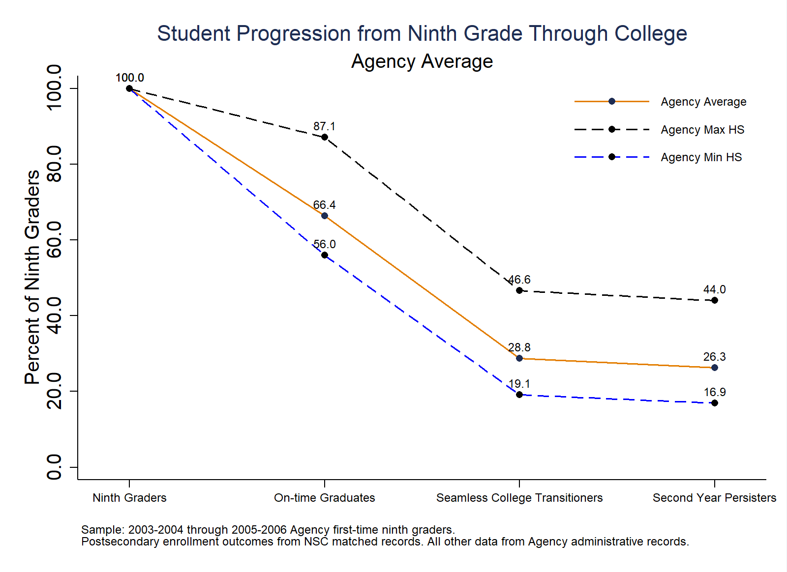
Purpose: This analysis tracks the overall percent of ninth graders who complete high school on-time, seamlessly enroll in college, and persist to the second year of college. To examine the range of attainment at each milestone, the minimum and maximum values of any high school are shown.
Required Analysis File Variables:
sidchrt_ninthfirst_hs_nameontime_gradenrl_1oct_ninth_yr1_anyenrl_1oct_ninth_yr2_anyAnalysis-Specific Sample Restrictions: Keep students in ninth grade cohorts for which persistence to the second year of college can be reported.
Ask Yourself
Analytic Technique: Calculate the proportion of first-time ninth graders that progress to each step along the education pipeline.
// Overall Progression

// Step 1: Load the college-going analysis file into Stata
use "$data/college_going_analysis", clear

// Step 2: Keep students in ninth grade cohorts you can observe persisting to the second year of college
local chrt_ninth_begin = ${chrt_ninth_begin_persist_yr2}
local chrt_ninth_end = ${chrt_ninth_end_persist_yr2}
keep if (chrt_ninth >= `chrt_ninth_begin' & chrt_ninth <= `chrt_ninth_end')

// Step 3: Create variables for the outcomes "regular diploma recipients", "seamless transitioners" and "second year persisters"
gen grad = (!mi(chrt_grad) & ontime_grad == 1)
gen seamless_transitioners_any = (enrl_1oct_ninth_yr1_any == 1 & ontime_grad == 1)
gen second_year_persisters = (enrl_1oct_ninth_yr1_any == 1 & enrl_1oct_ninth_yr2_any == 1 & ontime_grad == 1)

// Step 4: Create agency-level average outcomes
// 1. Preserve the data (to work with the data in its existing structure later on)
preserve

// 2. Calculate the mean of each outcome variable by agency
    collapse (mean) grad seamless_transitioners_any second_year_persisters (count) N = sid

// 3. Create a string variable called school_name equal to "${agency_name} Average"
    gen school_name = "${agency_name} AVERAGE"

// 4. Save this data as a temporary file
    tempfile agency_level
    save `agency_level'

// 5. Restore the data to the original form
restore

// Step 5: Create school-level maximum and minimum outcomes
// 1. Create a variable school_name that takes on the value of studentsҠfirst high school attended
gen school_name = first_hs_name
// 2. Calculate the mean of each outcome variable by first high school attended
collapse (mean) grad seamless_transitioners second_year_persisters (count) N = sid, by(school_name)

// 3. Identify the agency maximum values for each of the three outcome variables
preserve
    collapse (max) grad seamless_transitioners_any second_year_persisters (count) N
    gen school_name = "${agency_name} MAX HS"

    tempfile agency_max
    save `agency_max'
restore

// 4. Identify the agency minimum values for each of the three outcome variables
preserve
    collapse (min) grad seamless_transitioners_any second_year_persisters (count) N
    gen school_name = "${agency_name} MIN HS"

    tempfile agency_min
    save `agency_min'
restore

// 5. Append the three tempfiles to the school-level file loaded into Stata
append using `agency_level'
append using `agency_max'
append using `agency_min'

// Step 6: Format the outcome variables so they read as percentages in the graph
foreach var of varlist grad seamless_transitioners_any second_year_persisters {
    replace `var' = (`var' * 100)
    format `var' %9.1f
}

// Step 7: Reformat the data file so that one variable contains all the outcomes of interest
// 1. Create 4 observations for each school: ninth grade, hs graduation, seamless college transition and second-year persistence
foreach i of numlist 1/4 {
    gen time`i' = `i'
}

// 2. Reshape the data file from wide to long
reshape long time , i(school_name N)
drop _j

// 3. Create a single variable that takes on all the outcomes of interest
bysort school_name: gen outcome = 100 if time == 1
bysort school_name: replace outcome = grad if time == 2
bysort school_name: replace outcome = seamless_transitioners_any if time == 3
bysort school_name: replace outcome = second_year_persisters if time == 4
format outcome %9.1f

// Step 8: Prepare to graph the results
// 1. Label the outcome
label define outcome 1 "Ninth Graders" 2 "On-time Graduates" ///
3 "Seamless College Transitioners" 4 "Second Year Persisters"
label values time outcome

// 2. Generate a cohort label to be used in the footnote for the graph
local temp_begin = `chrt_ninth_begin'-1
local temp_end = `chrt_ninth_end'-1
if `chrt_ninth_begin'==`chrt_ninth_end' {
        local chrt_label "`temp_begin'-`chrt_ninth_begin'"
}
else {
        local chrt_label "`temp_begin'-`chrt_ninth_begin' through `temp_end'-`chrt_ninth_end'"
}

// Step 9: Graph the results
#delimit ;
twoway (connected outcome time if school_name == "${agency_name} AVERAGE",
        sort lcolor(dkorange) mlabel(outcome) mlabc(black) mlabs(vsmall) mlabp(12)
        mcolor(dknavy) msymbol(circle) msize(small))
        (connected outcome time if school_name == "${agency_name} MAX HS", sort lcolor(black)
        lpattern(dash) mlabel(outcome) mlabs(vsmall) mlabp(12) mlabc(black)
        mcolor(black) msize(small))
        (connected outcome time if school_name == "${agency_name} MIN HS", sort lcolor(blue)
        lpattern(dash) mlabel(outcome) mlabs(vsmall) mlabp(12) mlabc(black)
        mcolor(black) msize(small)),
title("Student Progression from Ninth Grade Through College", size(medium))
        subtitle("${agency_name} Average", size(medsmall))
        xscale(range(.8(.2)4.2))
        xtitle("") xlabel(1 2 3 4 , valuelabels labsize(vsmall))
        ytitle("Percent of Ninth Graders")
        yscale(range(0(20)100))
        ylabel(0(20)100, nogrid)
legend(col(1) position(2) size(vsmall)
        label(1 "${agency_name} Average")
        label(2 "${agency_name} Max HS")
        label(3 "${agency_name} Min HS")
        ring(0) region(lpattern(none) lcolor(none) fcolor(none)))
graphregion(color(white) fcolor(white) lcolor(white))
plotregion(color(white) fcolor(white) lcolor(white))
note(" " "Sample: `chrt_label' ${agency_name} first-time ninth graders." "Postsecondary enrollment outcomes from NSC matched records. All other data from ${agency_name} administrative records.", size(vsmall));
#delimit cr

graph export "$figures/A1_Overall_Progression.png", replace width(1600) height(1200)
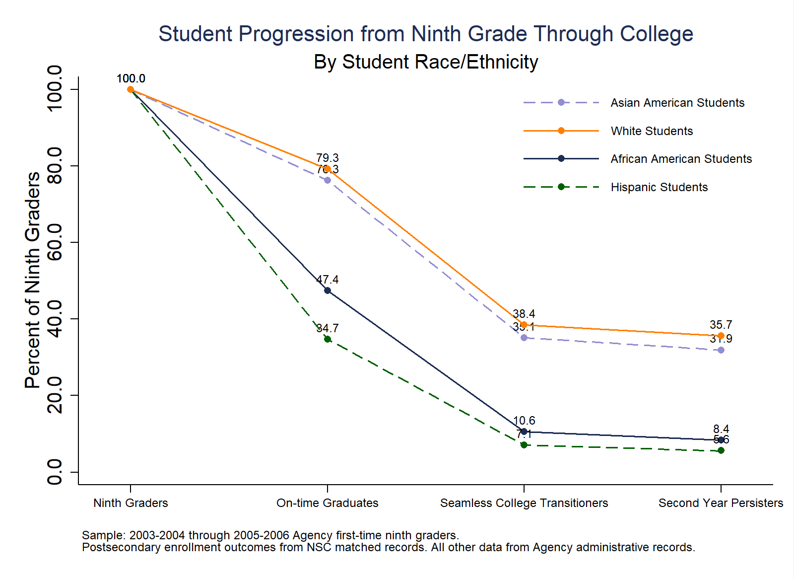
Purpose: This analysis tracks the percent of ninth graders of different races/ethnicities who complete high school on-time, seamlessly enroll in college, and persist to the second year of college.
Required Analysis File Variables:
sidrace_ethnicitychrt_ninthontime_gradenrl_1oct_ninth_yr1_anyenrl_1oct_ninth_yr2_anyAnalysis-Specific Sample Restrictions:
Ask Yourself
Analytic Technique: Calculate the proportion of first-time ninth graders that progress to each step along the education pipeline.
// Progression by Student Race/Ethnicity

// Step 1: Load the college-going analysis file into Stata
use "$data/college_going_analysis", clear

// Step 2: Keep students in ninth grade cohorts you can observe persisting to the second year of college
local chrt_ninth_begin = ${chrt_ninth_begin_persist_yr2}
local chrt_ninth_end = ${chrt_ninth_end_persist_yr2}
keep if (chrt_ninth >= `chrt_ninth_begin' & chrt_ninth <= `chrt_ninth_end')

// Step 3: Create variables for the outcomes "regular diploma recipients", "seamless transitioners" and "second year persisters"
gen grad = (!mi(chrt_grad) & ontime_grad == 1)
gen seamless_transitioners_any = (enrl_1oct_ninth_yr1_any == 1 & ontime_grad == 1)
gen second_year_persisters = (enrl_1oct_ninth_yr1_any == 1 & enrl_1oct_ninth_yr2_any == 1 & ontime_grad == 1)

// Step 4: Create average outcomes by race/ethnicity
collapse (mean) grad seamless_transitioners_any second_year_persisters (count) N=sid, ///
by(race_ethnicity)

// Step 5: Format the outcome variables so they read as percentages in the graph
foreach var of varlist grad seamless_transitioners_any second_year_persisters {
    replace `var' = (`var' * 100)
    format `var' %9.1f
}

// Step 6: Reformat the data file so that one variable contains all the outcomes of interest
// 1. Create 4 observations for each school: ninth grade, hs graduation, seamless college transition and second-year persistence
foreach i of numlist 1/4 {
    gen time`i' = `i'
}

// 2. Keep only African-American, Asian-American, Hispanic, and White students
keep if race_ethnicity == 1 | race_ethnicity == 2 | race_ethnicity == 3 | race_ethnicity == 5
sort race_ethnicity
gen sortorder = _n

// 3. Reshape the data file from wide to long
reshape long time , i(sortorder)

// 4. Create a single variable that takes on all the outcomes of interest
bysort race_ethnicity: gen outcome = 100 if time == 1
bysort race_ethnicity: replace outcome = grad if time == 2
bysort race_ethnicity: replace outcome = seamless_transitioners_any if time == 3
bysort race_ethnicity: replace outcome = second_year_persisters if time == 4
format outcome %9.1f

// Step 7: Prepare to graph the results
// 1. Label the outcome
label define outcome 1 "Ninth Graders" 2 "On-time Graduates" ///
3 "Seamless College Transitioners" 4 "Second Year Persisters"
label values time outcome

// 2. Generate a cohort label to be used in the footnote for the graph
local temp_begin = `chrt_ninth_begin'-1
local temp_end = `chrt_ninth_end'-1
if `chrt_ninth_begin'==`chrt_ninth_end' {
        local chrt_label "`temp_begin'-`chrt_ninth_begin'"
}
else {
        local chrt_label "`temp_begin'-`chrt_ninth_begin' through `temp_end'-`chrt_ninth_end'"
}

// Step 8: Graph the results
#delimit;
twoway (connected outcome time if race_ethnicity==1,
        sort lcolor(dknavy) mlabel(outcome) mlabc(black)mlabs(vsmall) mlabp(12)
        mcolor(dknavy) msymbol(circle) msize(small))
        (connected outcome time if race_ethnicity==2 , sort lcolor(lavender) lpattern(dash)
        mlabel(outcome) mlabs(vsmall) mlabp(12) mlabc(black) mcolor(lavender) msize(small))
        (connected outcome time if race_ethnicity==3 , sort lcolor(dkgreen) lpattern(dash)
        mlabel(outcome) mlabs(vsmall) mlabp(12) mlabc(black) mcolor(dkgreen) msize(small))
        (connected outcome time if race_ethnicity==5 , sort lcolor(orange) mlabel(outcome) mlabc(black)
        mlabs(vsmall) mlabp(12) mcolor(orange) msymbol(circle) msize(small)),
title("Student Progression from Ninth Grade Through College", size(medium))
        subtitle("By Student Race/Ethnicity", size(medsmall))
        xscale(range(.8(.2)4.2))
        xlabel(1 2 3 4 , valuelabels labsize(vsmall))
        ytitle("Percent of Ninth Graders")
        yscale(range(0(20)100))
        ylabel(0(20)100, nogrid)
        xtitle("", color(white))
legend(order(2 4 1 3) col(1) position(2) size(vsmall)
        label(1 "African American Students")
        label(2 "Asian American Students")
        label(3 "Hispanic Students")
        label(4 "White Students")
        ring(0) region(lpattern(none) lcolor(none) fcolor(none)))
graphregion(color(white) fcolor(white) lcolor(white))
plotregion(color(white) fcolor(white) lcolor(white))
note(" " "Sample: `chrt_label' ${agency_name} first-time ninth graders." "Postsecondary enrollment outcomes from NSC matched records. All other data from ${agency_name} administrative records." , size(vsmall));
#delimit cr

graph export "$figures/A2_Progression_by_RaceEthnicity.png", replace width(1600) height(1200)
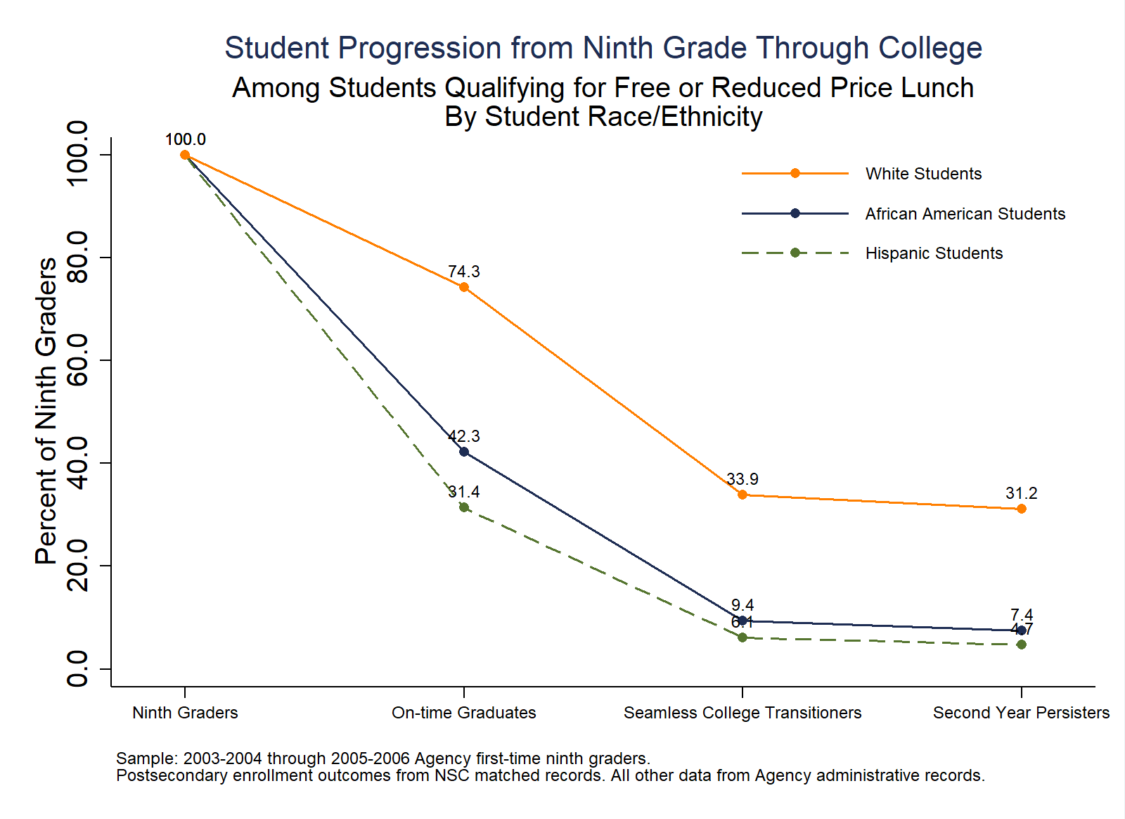
Purpose: This analysis tracks the percent of ninth graders of different races/ethnicities who ever qualified for free or reduce price lunch who complete high school on-time, seamlessly enroll in college, and persist to the second year of college.
Required Analysis File Variables:
sidrace_ethnicityfrpl_everchrt_ninthontime_gradenrl_1oct_ninth_yr1_anyenrl_1oct_ninth_yr2_anyAnalysis-Specific Sample Restrictions:
Ask Yourself
Analytic Technique: Calculate the proportion of first-time ninth graders that progress to each step along the education pipeline.
// Progression by Student Race/Ethnicity, Among FRPL Students

// Step 1: Load the college-going analysis file into Stata
use "$data/college_going_analysis", clear

// Step 2: Keep students in ninth grade cohorts you can observe persisting to the second year of college AND are ever FRPL-eligible
local chrt_ninth_begin = ${chrt_ninth_begin_persist_yr2}
local chrt_ninth_end = ${chrt_ninth_end_persist_yr2}
keep if (chrt_ninth >= `chrt_ninth_begin' & chrt_ninth <= `chrt_ninth_end')
keep if frpl_ever == 1

// Next, repeat steps 3-9 from the previous analysis
// Step 3: Create variables for the outcomes "regular diploma recipients", "seamless transitioners" and "second year persisters" .
gen grad = (!mi(chrt_grad) & ontime_grad == 1)
gen seamless_transitioners_any = (enrl_1oct_ninth_yr1_any == 1 & ontime_grad == 1)
gen second_year_persisters = (enrl_1oct_ninth_yr1_any == 1 & enrl_1oct_ninth_yr2_any == 1 & ontime_grad == 1)

// Step 4: Create average outcomes by race/ethnicity and drop any race/ethnic groups with fewer than 20 students
collapse (mean) grad seamless_transitioners_any second_year_persisters (count) N=sid, by(race_ethnicity)
drop if N < 20

// Step 5: Format the outcome variables so they read as percentages in the graph
foreach var of varlist grad seamless_transitioners_any second_year_persisters {
    replace `var' = (`var' * 100)
    format `var' %9.1f
}

// Step 6: Reformat the data file so that one variable contains all the outcomes of interest
// 1. Create 4 observations for each school: ninth grade, hs graduation, seamless college transition and second-year persistence
foreach i of numlist 1/4 {
    gen time`i' = `i'
}

// 2. Keep only African American, Asian American, Hispanic, and White students
keep if race_ethnicity == 1 | race_ethnicity == 2 | race_ethnicity == 3 | race_ethnicity == 5
sort race_ethnicity
gen sortorder = _n

// 3. Reshape the data file from wide to long
reshape long time , i(sortorder)

// 4. Create a single variable that takes on all the outcomes of interest
bysort race_ethnicity: gen outcome = 100 if time == 1
bysort race_ethnicity: replace outcome = grad if time == 2
bysort race_ethnicity: replace outcome = seamless_transitioners_any if time == 3
bysort race_ethnicity: replace outcome = second_year_persisters if time == 4
format outcome %9.1f

// Step 7: Prepare to graph the results
// 1. Label the outcome
label define outcome 1 "Ninth Graders" 2 "On-time Graduates" ///
3 "Seamless College Transitioners" 4 "Second Year Persisters"
label values time outcome

// 2. Generate a cohort label to be used in the footnote for the graph
local temp_begin = `chrt_ninth_begin'-1
local temp_end = `chrt_ninth_end'-1
if `chrt_ninth_begin'==`chrt_ninth_end' {
        local chrt_label "`temp_begin'-`chrt_ninth_begin'"
}
else {
        local chrt_label "`temp_begin'-`chrt_ninth_begin' through `temp_end'-`chrt_ninth_end'"
}

// Step 8: Graph the results
#delimit ;
twoway (connected outcome time if race_ethnicity==1 , sort lcolor(dknavy) mlabel(outcome)
        mlabc(black) mlabs(vsmall) mlabp(12) mcolor(dknavy) msymbol(circle) msize(small))
        (connected outcome time if race_ethnicity==3 , sort lcolor(forest_green) lpattern(dash)
        mlabel(outcome) mlabs(vsmall) mlabp(12) mlabc(black) mcolor(forest_green) msize(small))
        (connected outcome time if race_ethnicity==5 , sort lcolor(orange) mlabel(outcome) mlabc(black)
        mlabs(vsmall) mlabp(12) mcolor(orange) msymbol(circle) msize(small)),
title("Student Progression from Ninth Grade Through College", size(medium))
        subtitle("Among Students Qualifying for Free or Reduced Price Lunch" "By Student Race/Ethnicity", size(medsmall))
        xscale(range(.8(.2)4.2))
        xlabel(1 2 3 4, valuelabels labsize(vsmall))
        ytitle("Percent of Ninth Graders")
        yscale(range(0(20)100))
        ylabel(0(20)100, nogrid)
        xtitle("", color(white))
legend(order(3 1 2) col(1) position(2) size(vsmall)
        label(1 "African American Students")
        label(2 "Hispanic Students")
        label(3 "White Students")
        ring(0) region(lpattern(none) lcolor(none) fcolor(none)))
graphregion(color(white) fcolor(white) lcolor(white))
plotregion(color(white) fcolor(white) lcolor(white))
note(" " "Sample: `chrt_label' ${agency_name} first-time ninth graders." "Postsecondary enrollment outcomes from NSC matched records. All other data from ${agency_name} administrative records." , size(vsmall));
#delimit cr

graph export "$figures/A3_Progression_by_RaceEthnicity_Frpl.png", replace width(1600) height(1200)
Purpose: This analysis tracks the percent of ninth graders at different levels of being on-track for graduation who complete high school on-time, seamlessly enroll in college, and then persist to the second year of college.
Required Analysis File Variables:
sidchrt_ninthontrack_sampleontrack_end_yr*cum_gpa_yr*ontime_gradenrl_1oct_ninth_yr1_anyenrl_1oct_ninth_yr2_anyAnalysis-Specific Sample Restrictions:
Ask Yourself
Analytic Technique: Calculate the proportion of first-time ninth graders that progressed along the education pipeline.

// Progression by Students' On-Track Status After Ninth Grade

// Step 1: Load the college-going analysis file into Stata
use "$data/college_going_analysis", clear

// Step 2: Keep students in ninth grade cohorts you can observe persisting to the second year of college AND are included in the on-track analysis sample
local chrt_ninth_begin = ${chrt_ninth_begin_persist_yr2}
local chrt_ninth_end = ${chrt_ninth_end_persist_yr2}
keep if (chrt_ninth >= `chrt_ninth_begin' & chrt_ninth <= `chrt_ninth_end')
keep if ontrack_sample == 1

// Step 3: Generate on-track indicators that take into account studentsҠGPAs upon completion of their first year in high school
label define ot 1 "Off-Track to Graduate" ///
2 "On-Track to Graduate, GPA < 3.0" ///
3 "On-Track to Graduate, GPA >= 3.0", replace

gen ontrack_endyr1_gpa = .
replace ontrack_endyr1_gpa = 1 if ontrack_endyr1 == 1
replace ontrack_endyr1_gpa = 2 if ontrack_endyr1 == 2 & cum_gpa_yr1 < 3 & !mi(cum_gpa_yr1)
replace ontrack_endyr1_gpa = 3 if ontrack_endyr1 == 2 & cum_gpa_yr1 >= 3 & !mi(cum_gpa_yr1)

assert !mi(ontrack_endyr1_gpa) if !mi(ontrack_endyr1) & !mi(cum_gpa_yr1)
label values ontrack_endyr1_gpa ot

// Step 4: Create variables for the outcomes "regular diploma recipients", "seamless transitioners" and "second year persisters"
gen grad = (!mi(chrt_grad) & ontime_grad == 1)
gen seamless_transitioners_any = (enrl_1oct_ninth_yr1_any == 1 & ontime_grad == 1)
gen second_year_persisters = (enrl_1oct_ninth_yr1_any == 1 & enrl_1oct_ninth_yr2_any == 1 & ontime_grad == 1)

// Step 5: Create average outcomes by on-track status at the end of ninth grade
collapse (mean) grad seamless_transitioners_any second_year_persisters (count) N=sid, ///
by(ontrack_endyr1_gpa)

// Step 6: Format the outcome variables so they read as percentages in the graph
foreach var of varlist grad seamless_transitioners_any second_year_persisters {
    replace `var' = (`var' * 100)
    format `var' %9.1f
}

// Step 7: Reformat the data file so that one variable contains all the outcomes of interest
// 1. Create 4 observations for each school: ninth grade, hs graduation, seamless college transition and second-year persistence
foreach i of numlist 1/4 {
    gen time`i' = `i'
}

// 2. Reshape the data file from wide to long
reshape long time, i(ontrack_endyr1_gpa N)

// 3. Create a single variable that takes on all the outcomes of interest
bysort ontrack_endyr1_gpa: gen outcome = 100 if time == 1
bysort ontrack_endyr1_gpa: replace outcome = grad if time == 2
bysort ontrack_endyr1_gpa: replace outcome = seamless_transitioners_any if time == 3
bysort ontrack_endyr1_gpa: replace outcome = second_year_persisters if time == 4
format outcome %9.1f

// Step 8: Prepare to graph the results
// 1. Label the outcome
label define outcome 1 "Ninth Graders" 2 "On-time Graduates" ///
3 "Seamless College Transitioners" 4 "Second Year Persisters"
label values time outcome

// 2. Generate a cohort label to be used in the footnote for the graph
local temp_begin = `chrt_ninth_begin'-1
local temp_end = `chrt_ninth_end'-1
if `chrt_ninth_begin'==`chrt_ninth_end' {
        local chrt_label "`temp_begin'-`chrt_ninth_begin'"
}
else {
        local chrt_label "`temp_begin'-`chrt_ninth_begin' through `temp_end'-`chrt_ninth_end'"
}

// Step 9: Graph the results
#delimit ;
twoway (connected outcome time if ontrack_endyr1_gpa == 1,
        sort lcolor(dkorange) mlabel(outcome) mlabc(black) mlabs(vsmall) mlabp(3)
        mcolor(dkorange) msymbol(circle) msize(small))
        (connected outcome time if ontrack_endyr1_gpa == 2, sort lcolor(navy*.6)
        mlabel(outcome) mlabs(vsmall) mlabp(3) mlabc(black) mcolor(navy*.6)
        msymbol(square) msize(small))
        (connected outcome time if ontrack_endyr1_gpa == 3, sort lcolor(navy*.9)
        mlabel(outcome) mlabs(vsmall) mlabp(3) mlabc(black) mcolor(navy*.9)
        msymbol(diamond) msize(small))
        (connected outcome time if ontrack_endyr1_gpa == 4, sort lcolor(navy*.3)
        mlabel(outcome) mlabs(vsmall) mlabp(3) mlabc(black) mcolor(navy*.3)
        msymbol(triangle) msize(small)),
title("Student Progression from Ninth Grade Through College", size(medium))
        ylabel(, nogrid)
        subtitle("By Course Credits and GPA after First High School Year", size(medsmall))
        xscale(range(.8(.2)4.2)) xlabel(1 2 3 4, valuelabels labsize(vsmall)) xtitle("")
        yscale(range(0(20)100)) ylabel(0(20)100, labsize(small) format(%9.0f))
        ytitle("Percent of Ninth Graders" " ")
legend(order(3 2 1) col(1) position(1) size(vsmall)
        label(1 "Off-Track to Graduate")
        label(2 "On-Track to Graduate, GPA<3.0")
        label(3 "On-Track to Graduate, GPA>=3.0")
        ring(0) region(lpattern(none) lcolor(none) fcolor(none)))
graphregion(color(white) fcolor(white) lcolor(white))
plotregion(color(white) fcolor(white) lcolor(white))
note(" " "Sample: `chrt_label' ${agency_name} first-time ninth graders. Students who transferred into or out of ${agency_name} are excluded" "from the sample. Postsecondary enrollment outcomes from NSC matched records. All other data are from ${agency_name} administrative records.", span size(vsmall));
#delimit cr

graph export "$figures/A4_Progression_by_OnTrack_Ninth.png", replace width(1600) height(1200)